set of eigenvalues, taking multiplicities into account

(0.004 seconds)

1—10 of 633 matching pages

2: 1.18 Linear Second Order Differential Operators and Eigenfunction Expansions

… ►If an eigenvalue has multiplicity

>1

, the eigenfunctions may always be orthogonalized in this degenerate sub-space. … ►For

\mathcal{D}(T)

we can take

C^{2}(X)

, with appropriate boundary conditions, and with compact support if

X

is bounded, which space is dense in

L^{2}\left(X\right)

, and for

X

unbounded require that possible non- $L^{2}$ eigenfunctions of (1.18.28), with real eigenvalues, are non-zero but bounded on open intervals, including

\pm\infty

. ►Stated informally, the spectrum of

T

is the set of it’s eigenvalues, these being real as

T

is self-adjoint. … … ►If an eigenvalue is of multiplicity greater than

1

then an orthonormal basis of eigenfunctions can be given for the eigenspace. …

3: 28.2 Definitions and Basic Properties

… ►

§28.2(v) Eigenvalues $a_{n}$ , $b_{n}$

►For given

\nu

and

q

, equation (28.2.16) determines an infinite discrete set of values of

a

, the eigenvalues or characteristic values, of Mathieu’s equation. When

\widehat{\nu}=0

1

, the notation for the two sets of eigenvalues corresponding to each

\widehat{\nu}

is shown in Table 28.2.1, together with the boundary conditions of the associated eigenvalue problem. … ►

Distribution

… ►

Change of Sign of $q$

…

… ►The mathematical project team has endeavored to take into account the hundreds of research papers and numerous books on special functions that have appeared since 1964. … ►In addition, there is a comprehensive account of the great variety of analytical methods that are used for deriving and applying the extremely important asymptotic properties of the special functions, including double asymptotic properties (Chapter 2 and §§10.41(iv), 10.41(v)). … ► ►►►►►

$(a,b]$ or $[a,b)$	half-closed intervals.
…
$\setminus$	set subtraction.
$\mathbb{Z}$	set of all integers.
$n\mathbb{Z}$	set of all integer multiples of $n$ .

…

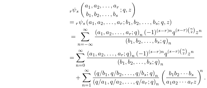
5: 17.4 Basic Hypergeometric Functions

… ►Here and elsewhere it is assumed that the

b_{j}

do not take any of the values

q^{-n}

. … ►

17.4.3

{{}_{r}\psi_{s}}\left({a_{1},a_{2},\dots,a_{r}\atop b_{1},b_{2},\dots,b_{s}};q% ,z\right)={{}_{r}\psi_{s}}\left(a_{1},a_{2},\dots,a_{r};b_{1},b_{2},\dots,b_{s% };q,z\right)=\sum_{n=-\infty}^{\infty}\frac{\left(a_{1},a_{2},\dots,a_{r};q% \right)_{n}(-1)^{(s-r)n}q^{(s-r)\genfrac{(}{)}{0.0pt}{}{n}{2}}z^{n}}{\left(b_{% 1},b_{2},\dots,b_{s};q\right)_{n}}=\sum_{n=0}^{\infty}\frac{\left(a_{1},a_{2},% \dots,a_{r};q\right)_{n}(-1)^{(s-r)n}q^{(s-r)\genfrac{(}{)}{0.0pt}{}{n}{2}}z^{% n}}{\left(b_{1},b_{2},\dots,b_{s};q\right)_{n}}+\sum_{n=1}^{\infty}\frac{\left% (q/b_{1},q/b_{2},\dots,q/b_{s};q\right)_{n}}{\left(q/a_{1},q/a_{2},\dots,q/a_{% r};q\right)_{n}}\left(\frac{b_{1}b_{2}\cdots b_{s}}{a_{1}a_{2}\cdots a_{r}z}% \right)^{n}.

ⓘ

Defines:: ${{}_{\NVar{r}}\psi_{\NVar{s}}}\left(\NVar{a_{1},\dots,a_{r}};\NVar{b_{1},\dots% ,b_{s}};\NVar{q},\NVar{z}\right)$ or ${{}_{\NVar{r}}\psi_{\NVar{s}}}\left({\NVar{a_{1},\dots,a_{r}}\atop\NVar{b_{1},% \dots,b_{s}}};\NVar{q},\NVar{z}\right)$ : bilateral basic hypergeometric (or bilateral $q$ -hypergeometric) function
Symbols:: $\genfrac{(}{)}{0.0pt}{}{\NVar{m}}{\NVar{n}}$ : binomial coefficient, $\left(\NVar{a_{1},a_{2},\dots,a_{r}};\NVar{q}\right)_{\NVar{n}}$ : multiple $q$ -Pochhammer symbol, $q$ : complex base, $n$ : nonnegative integer, $r$ : nonnegative integer, $s$ : nonnegative integer and $z$ : complex variable
Permalink:: http://dlmf.nist.gov/17.4.E3
Encodings:: pMML, png, TeX
See also:: Annotations for §17.4(ii), §17.4 and Ch.17

►Here and elsewhere the

b_{j}

must not take any of the values

q^{-n}

, and the

a_{j}

must not take any of the values

q^{n+1}

. The infinite series converge when

s\geq r

provided that

|(b_{1}\cdots b_{s})/(a_{1}\cdots a_{r}z)|<1

and also, in the case

s=r

|z|<1

. … ►

17.4.6

\Phi^{(2)}\left(a;b,b^{\prime};c,c^{\prime};q;x,y\right)=\sum_{m,n\geq 0}\frac% {\left(a;q\right)_{m+n}\left(b;q\right)_{m}\left(b^{\prime};q\right)_{n}x^{m}y% ^{n}}{\left(q,c;q\right)_{m}\left(q,c^{\prime};q\right)_{n}},

ⓘ

Defines:: $\Phi^{(2)}\left(\NVar{a};\NVar{b},\NVar{b^{\prime}};\NVar{c},\NVar{c^{\prime}}% ;\NVar{q};\NVar{x},\NVar{y}\right)$ : second $q$ -Appell function
Symbols:: $\left(\NVar{a};\NVar{q}\right)_{\NVar{n}}$ : $q$ -Pochhammer symbol (or $q$ -shifted factorial), $\left(\NVar{a_{1},a_{2},\dots,a_{r}};\NVar{q}\right)_{\NVar{n}}$ : multiple $q$ -Pochhammer symbol, $q$ : complex base, $m$ : nonnegative integer, $n$ : nonnegative integer, $x$ : real variable and $y$ : real variable
Referenced by:: Erratum (V1.0.10) for Section 17.1, Erratum (V1.1.3) for Equation (17.4.6)
Permalink:: http://dlmf.nist.gov/17.4.E6
Encodings:: pMML, png, TeX
Clarification (effective with 1.1.3):: The explicit usage of $\left(q,c;q\right)_{m}\left(q,c^{\prime};q\right)_{n}$ in the denominator of the right-hand side was used.
Correction (effective with 1.0.10):: The notation for $\Phi^{(2)}$ has been updated to that of Gasper and Rahman (2004) to explicitly include the $q$ argument.
See also:: Annotations for §17.4(iii), §17.4 and Ch.17

…

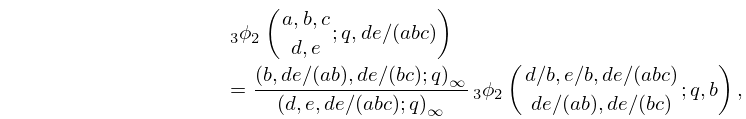
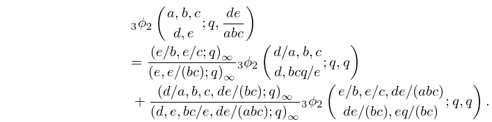
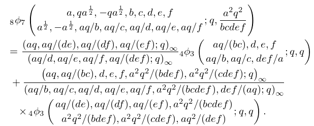
6: 17.9 Further Transformations of ${{}_{r+1}\phi_{r}}$ Functions

… ►

17.9.3_5

{{}_{2}\phi_{1}}\left({a,b\atop c};q,z\right)=\frac{\left(c/a,c/b;q\right)_{% \infty}}{\left(c,c/(ab);q\right)_{\infty}}{{}_{3}\phi_{2}}\left({a,b,abz/c% \atop qab/c,0};q,q\right)+\frac{\left(a,b,abz/c;q\right)_{\infty}}{\left(c,ab/% c,z;q\right)_{\infty}}{{}_{3}\phi_{2}}\left({c/a,c/b,z\atop qc/(ab),0};q,q% \right),

ⓘ

Symbols:: ${{}_{\NVar{r+1}}\phi_{\NVar{s}}}\left(\NVar{a_{0},\dots,a_{r}};\NVar{b_{1},% \dots,b_{s}};\NVar{q},\NVar{z}\right)$ or ${{}_{\NVar{r+1}}\phi_{\NVar{s}}}\left({\NVar{a_{0},\dots,a_{r}}\atop\NVar{b_{1% },\dots,b_{s}}};\NVar{q},\NVar{z}\right)$ : basic hypergeometric (or $q$ -hypergeometric) function, $\left(\NVar{a_{1},a_{2},\dots,a_{r}};\NVar{q}\right)_{\NVar{n}}$ : multiple $q$ -Pochhammer symbol, $q$ : complex base and $z$ : complex variable
Proof sketch:: Derivable from (17.9.13) after replacing $a$ with $d/a$ and then taking $d\rightarrow 0$ . Then replace $a$ , $b$ , $c$ , $e$ with $abz/c$ , $a$ , $b$ , $c$ respectively.
Referenced by:: §17.9(i), Erratum (V1.1.0) for Additions
Permalink:: http://dlmf.nist.gov/17.9.E3_5
Encodings:: pMML, png, TeX
Addition (effective with 1.1.0):: This equation was added.
See also:: Annotations for §17.9(i), §17.9(i), §17.9 and Ch.17

… ►

17.9.7

{{}_{3}\phi_{2}}\left({a,b,c\atop d,e};q,de/(abc)\right)=\frac{\left(b,de/(ab)% ,de/(bc);q\right)_{\infty}}{\left(d,e,de/(abc);q\right)_{\infty}}\*{{}_{3}\phi% _{2}}\left({d/b,e/b,de/(abc)\atop de/(ab),de/(bc)};q,b\right),

ⓘ

Symbols:: ${{}_{\NVar{r+1}}\phi_{\NVar{s}}}\left(\NVar{a_{0},\dots,a_{r}};\NVar{b_{1},% \dots,b_{s}};\NVar{q},\NVar{z}\right)$ or ${{}_{\NVar{r+1}}\phi_{\NVar{s}}}\left({\NVar{a_{0},\dots,a_{r}}\atop\NVar{b_{1% },\dots,b_{s}}};\NVar{q},\NVar{z}\right)$ : basic hypergeometric (or $q$ -hypergeometric) function, $\left(\NVar{a_{1},a_{2},\dots,a_{r}};\NVar{q}\right)_{\NVar{n}}$ : multiple $q$ -Pochhammer symbol and $q$ : complex base
Permalink:: http://dlmf.nist.gov/17.9.E7
Encodings:: pMML, png, TeX
See also:: Annotations for §17.9(ii), §17.9(ii), §17.9 and Ch.17

… ►

17.9.13

{{}_{3}\phi_{2}}\left({a,b,c\atop d,e};q,\frac{de}{abc}\right)=\frac{\left(e/b% ,e/c;q\right)_{\infty}}{\left(e,e/(bc);q\right)_{\infty}}{{}_{3}\phi_{2}}\left% ({d/a,b,c\atop d,bcq/e};q,q\right)+\frac{\left(d/a,b,c,de/(bc);q\right)_{% \infty}}{\left(d,e,bc/e,de/(abc);q\right)_{\infty}}{{}_{3}\phi_{2}}\left({e/b,% e/c,de/(abc)\atop de/(bc),eq/(bc)};q,q\right).

ⓘ

Symbols:: ${{}_{\NVar{r+1}}\phi_{\NVar{s}}}\left(\NVar{a_{0},\dots,a_{r}};\NVar{b_{1},% \dots,b_{s}};\NVar{q},\NVar{z}\right)$ or ${{}_{\NVar{r+1}}\phi_{\NVar{s}}}\left({\NVar{a_{0},\dots,a_{r}}\atop\NVar{b_{1% },\dots,b_{s}}};\NVar{q},\NVar{z}\right)$ : basic hypergeometric (or $q$ -hypergeometric) function, $\left(\NVar{a_{1},a_{2},\dots,a_{r}};\NVar{q}\right)_{\NVar{n}}$ : multiple $q$ -Pochhammer symbol and $q$ : complex base
Referenced by:: (17.9.3_5)
Permalink:: http://dlmf.nist.gov/17.9.E13
Encodings:: pMML, png, TeX
See also:: Annotations for §17.9(ii), §17.9(ii), §17.9 and Ch.17

… ►

17.9.14

{{}_{4}\phi_{3}}\left({q^{-n},a,b,c\atop d,e,f};q,q\right)=\frac{\left(e/a,f/a% ;q\right)_{n}}{\left(e,f;q\right)_{n}}a^{n}{{}_{4}\phi_{3}}\left({q^{-n},a,d/b% ,d/c\atop d,aq^{1-n}/e,aq^{1-n}/f};q,q\right)=\frac{\left(a,ef/(ab),ef/(ac);q% \right)_{n}}{\left(e,f,ef/(abc);q\right)_{n}}{{}_{4}\phi_{3}}\left({q^{-n},e/a% ,f/a,ef/(abc)\atop ef/(ab),ef/(ac),q^{1-n}/a};q,q\right).

ⓘ

Symbols:: ${{}_{\NVar{r+1}}\phi_{\NVar{s}}}\left(\NVar{a_{0},\dots,a_{r}};\NVar{b_{1},% \dots,b_{s}};\NVar{q},\NVar{z}\right)$ or ${{}_{\NVar{r+1}}\phi_{\NVar{s}}}\left({\NVar{a_{0},\dots,a_{r}}\atop\NVar{b_{1% },\dots,b_{s}}};\NVar{q},\NVar{z}\right)$ : basic hypergeometric (or $q$ -hypergeometric) function, $\left(\NVar{a_{1},a_{2},\dots,a_{r}};\NVar{q}\right)_{\NVar{n}}$ : multiple $q$ -Pochhammer symbol, $q$ : complex base and $n$ : nonnegative integer
Permalink:: http://dlmf.nist.gov/17.9.E14
Encodings:: pMML, png, TeX
See also:: Annotations for §17.9(iii), §17.9(iii), §17.9 and Ch.17

… ►

17.9.16

{{}_{8}\phi_{7}}\left({a,qa^{\frac{1}{2}},-qa^{\frac{1}{2}},b,c,d,e,f\atop a^{% \frac{1}{2}},-a^{\frac{1}{2}},aq/b,aq/c,aq/d,aq/e,aq/f};q,\frac{a^{2}q^{2}}{% bcdef}\right)=\frac{\left(aq,aq/(de),aq/(df),aq/(ef);q\right)_{\infty}}{\left(% aq/d,aq/e,aq/f,aq/(def);q\right)_{\infty}}{{}_{4}\phi_{3}}\left({aq/(bc),d,e,f% \atop aq/b,aq/c,def/a};q,q\right)+\frac{\left(aq,aq/(bc),d,e,f,a^{2}q^{2}/(% bdef),a^{2}q^{2}/(cdef);q\right)_{\infty}}{\left(aq/b,aq/c,aq/d,aq/e,aq/f,a^{2% }q^{2}/(bcdef),def/(aq);q\right)_{\infty}}\*{{}_{4}\phi_{3}}\left({aq/(de),aq/% (df),aq/(ef),a^{2}q^{2}/(bcdef)\atop a^{2}q^{2}/(bdef),a^{2}q^{2}/(cdef),aq^{2% }/(def)};q,q\right).

ⓘ

Symbols:: ${{}_{\NVar{r+1}}\phi_{\NVar{s}}}\left(\NVar{a_{0},\dots,a_{r}};\NVar{b_{1},% \dots,b_{s}};\NVar{q},\NVar{z}\right)$ or ${{}_{\NVar{r+1}}\phi_{\NVar{s}}}\left({\NVar{a_{0},\dots,a_{r}}\atop\NVar{b_{1% },\dots,b_{s}}};\NVar{q},\NVar{z}\right)$ : basic hypergeometric (or $q$ -hypergeometric) function, $\left(\NVar{a_{1},a_{2},\dots,a_{r}};\NVar{q}\right)_{\NVar{n}}$ : multiple $q$ -Pochhammer symbol and $q$ : complex base
Permalink:: http://dlmf.nist.gov/17.9.E16
Encodings:: pMML, png, TeX
See also:: Annotations for §17.9(iii), §17.9(iii), §17.9 and Ch.17

…

7: Bille C. Carlson

… ►In theoretical physics he is known for the “Carlson-Keller Orthogonalization”, published in 1957, Orthogonalization Procedures and the Localization of Wannier Functions, and the “Carlson-Keller Theorem”, published in 1961, Eigenvalues of Density Matrices. … ►The main theme of Carlson’s mathematical research has been to expose previously hidden permutation symmetries that can eliminate a set of transformations and thereby replace many formulas by a few. … ►In Symmetry in c, d, n of Jacobian elliptic functions (2004) he found a previously hidden symmetry in relations between Jacobian elliptic functions, which can now take a form that remains valid when the letters c, d, and n are permuted. This invariance usually replaces sets of twelve equations by sets of three equations and applies also to the relation between the first symmetric elliptic integral and the Jacobian functions. …

8: 3.8 Nonlinear Equations

… ►Sometimes the equation takes the form … ►For multiple zeros the convergence is linear, but if the multiplicity

m

is known then quadratic convergence can be restored by multiplying the ratio

f(z_{n})/f^{\prime}(z_{n})

in (3.8.4) by

m

. … ►

Eigenvalue Methods

►For the computation of zeros of orthogonal polynomials as eigenvalues of finite tridiagonal matrices (§3.5(vi)), see Gil et al. (2007a, pp. 205–207). … ►It is called a Julia set. …

9: About Color Map

… ►In doing this, however, we would like to place the mathematically significant phase values, specifically the multiples of

\pi/2

correponding to the real and imaginary axes, at more immediately recognizable colors. … ►The conventional CMYK color wheel (not to be confused with the traditional Artist’s color wheel) places the additive colors (red, green, blue) and the subtractive colors (yellow, cyan, magenta) at multiples of 60 degrees. … ►We therefore use a piecewise linear mapping as illustrated below, that takes phase

0

to red,

\pi/2

to yellow,

\pi

to cyan and

3\pi/2

to blue. …

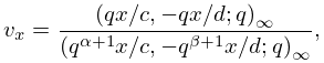
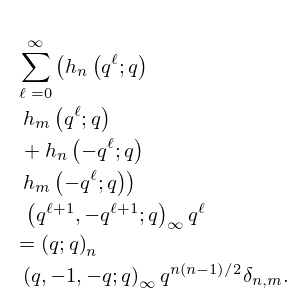
10: 18.27 $q$ -Hahn Class

… ►The

q

-Hahn class OP’s comprise systems of OP’s

\{p_{n}(x)\}

n=0,1,\dots,N

, or

n=0,1,2,\dots

, that are eigenfunctions of a second order

q

-difference operator. …where

A(x)

B(x)

, and

C(x)

are independent of

n

, and where the

\lambda_{n}

are the eigenvalues. In the

q

-Hahn class OP’s the role of the operator

\ifrac{\mathrm{d}}{\mathrm{d}x}

in the Jacobi, Laguerre, and Hermite cases is played by the

q

-derivative

\mathcal{D}_{q}

, as defined in (17.2.41). … ►

18.27.12

v_{x}=\frac{\left(qx/c,-qx/d;q\right)_{\infty}}{\left(q^{\alpha+1}x/c,-q^{% \beta+1}x/d;q\right)_{\infty}},

\alpha,\beta>-1

c,d>0

ⓘ

Symbols:: $\left(\NVar{a_{1},a_{2},\dots,a_{r}};\NVar{q}\right)_{\NVar{n}}$ : multiple $q$ -Pochhammer symbol, $q$ : real variable, $x$ : real variable and $v_{x}$
Permalink:: http://dlmf.nist.gov/18.27.E12
Encodings:: pMML, png, TeX
Correction (effective with 1.1.2):: $q$ -Pochhammer symbols now link to their definition.
See also:: Annotations for §18.27(iii), §18.27 and Ch.18

… ►

18.27.22

\sum_{\ell=0}^{\infty}\left(h_{n}\left(q^{\ell};q\right)h_{m}\left(q^{\ell};q% \right)+h_{n}\left(-q^{\ell};q\right)h_{m}\left(-q^{\ell};q\right)\right)\*% \left(q^{\ell+1},-q^{\ell+1};q\right)_{\infty}q^{\ell}=\left(q;q\right)_{n}% \left({q,-1,-q};q\right)_{\infty}q^{n(n-1)/2}\delta_{n,m}.

ⓘ

Symbols:: $\delta_{\NVar{j},\NVar{k}}$ : Kronecker delta, $h_{\NVar{n}}\left(\NVar{x};\NVar{q}\right)$ : discrete $q$ -Hermite I polynomial, $\left(\NVar{a};\NVar{q}\right)_{\NVar{n}}$ : $q$ -Pochhammer symbol (or $q$ -shifted factorial), $\left(\NVar{a_{1},a_{2},\dots,a_{r}};\NVar{q}\right)_{\NVar{n}}$ : multiple $q$ -Pochhammer symbol, $q$ : real variable, $\ell$ : nonnegative integer, $m$ : nonnegative integer and $n$ : nonnegative integer
Permalink:: http://dlmf.nist.gov/18.27.E22
Encodings:: pMML, png, TeX
See also:: Annotations for §18.27(vii), §18.27(vii), §18.27 and Ch.18

…

set of eigenvalues, taking multiplicities into account

1—10 of 633 matching pages

1: 3.2 Linear Algebra

§3.2(iv) Eigenvalues and Eigenvectors

§3.2(v) Condition of Eigenvalues

2: 1.18 Linear Second Order Differential Operators and Eigenfunction Expansions

3: 28.2 Definitions and Basic Properties

§28.2(v) Eigenvalues $a_{n}$ , $b_{n}$

Distribution

Change of Sign of $q$

4: Mathematical Introduction

5: 17.4 Basic Hypergeometric Functions

6: 17.9 Further Transformations of ${{}_{r+1}\phi_{r}}$ Functions

7: Bille C. Carlson

8: 3.8 Nonlinear Equations

Eigenvalue Methods

9: About Color Map

10: 18.27 $q$ -Hahn Class

set of eigenvalues, taking multiplicities into account

1—10 of 633 matching pages

1: 3.2 Linear Algebra

§3.2(iv) Eigenvalues and Eigenvectors

§3.2(v) Condition of Eigenvalues

2: 1.18 Linear Second Order Differential Operators and Eigenfunction Expansions

3: 28.2 Definitions and Basic Properties

§28.2(v) Eigenvalues a n , b n

Distribution

Change of Sign of q

4: Mathematical Introduction

5: 17.4 Basic Hypergeometric Functions

6: 17.9 Further Transformations of ϕ r r + 1 Functions

7: Bille C. Carlson

8: 3.8 Nonlinear Equations

Eigenvalue Methods

9: About Color Map

10: 18.27 q -Hahn Class

§28.2(v) Eigenvalues $a_{n}$ , $b_{n}$

Change of Sign of $q$

6: 17.9 Further Transformations of ${{}_{r+1}\phi_{r}}$ Functions

10: 18.27 $q$ -Hahn Class