reduced%20Planck%20constant

SearchAdvancedHelp

(0.003 seconds)

1—10 of 514 matching pages

1: 14.30 Spherical and Spheroidal Harmonics

… ►

14.30.11 $$L^2{Y}_{l,m}={\mathrm{\hslash }}^{2}l(l+1)Y_{l,m},$$ $l=0,1,2,\mathrm{\dots }$,

ⓘ

Symbols:

$Y_{l,m}(\theta ,\varphi )$: spherical harmonic, $m$: integer, $l$: nonnegative integer and $L$: angular momentum operator

Referenced by:

§18.39(ii)

Permalink:

http://dlmf.nist.gov/14.30.E11

Encodings:

pMML, png, TeX

See also:

Annotations for §14.30(iv), §14.30 and Ch.14

… ►

14.30.11_5 $${\mathrm{L}}_z{Y}_{l,m}=\mathrm{\hslash }m{Y}_{l,m},$$ $m=-l,-1+1,\mathrm{\dots },0,\mathrm{\dots },l-1,l$,

ⓘ

Symbols:

$Y_{l,m}(\theta ,\varphi )$: spherical harmonic, $m$: integer, $l$: nonnegative integer and ${\mathrm{L}}_z$: $z$ component of the angular momentum operator

Referenced by:

§14.30(iv), Erratum (V1.1.0) for Additions

Permalink:

http://dlmf.nist.gov/14.30.E11_5

Encodings:

pMML, png, TeX

Addition (effective with 1.1.0):

This equation was added.

See also:

Annotations for §14.30(iv), §14.30 and Ch.14

►where $\mathrm{\hslash }$ is the reduced Planck’s constant. … ►

14.30.12 $$L^2=-{\mathrm{\hslash }}^2\left(\frac{1}{\sin \theta }\frac{\partial }{\partial \theta }\left(\sin \theta \frac{\partial }{\partial \theta }\right)+\frac{1}{{\sin }^2\theta }\frac{{\partial }^2}{{\partial \varphi }^2}\right),$$

ⓘ

Defines:

$L$: angular momentum operator (locally)

Symbols:

$\frac{\partial f}{\partial x}$: partial derivative of $f$ with respect to $x$ , $\partial x$: partial differential of $x$ and $\sin z$: sine function

Referenced by:

§18.39(ii)

Permalink:

http://dlmf.nist.gov/14.30.E12

Encodings:

pMML, png, TeX

See also:

Annotations for §14.30(iv), §14.30 and Ch.14

… ►

14.30.13 $${\mathrm{L}}_z=-\mathrm{i}\mathrm{\hslash }\frac{\partial }{\partial \varphi };$$

ⓘ

Defines:

${\mathrm{L}}_z$: $z$ component of the angular momentum operator (locally)

Symbols:

$\mathrm{i}$: imaginary unit, $\frac{\partial f}{\partial x}$: partial derivative of $f$ with respect to $x$ , $\partial x$: partial differential of $x$ and $z$: complex variable

Referenced by:

§14.30(iv), Erratum (V1.1.0) for Additions

Permalink:

http://dlmf.nist.gov/14.30.E13

Encodings:

pMML, png, TeX

Addition (effective with 1.1.0):

This equation was added.

See also:

Annotations for §14.30(iv), §14.30 and Ch.14

…

2: 18.39 Applications in the Physical Sciences

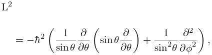
… ►where $x$ is a spatial coordinate, $m$ the mass of the particle with potential energy $V(x)$, $\mathrm{\hslash }=h/(2\pi )$ is the reduced Planck’s constant, and $(a,b)$ a finite or infinite interval. ►Here the term $-\frac{{\mathrm{\hslash }}^2}{2m}\frac{{\partial }^2}{{\partial x}^2}$ represents the quantum kinetic energy of a single particle of mass $m$, and $V(x)$ its potential energy. … ►and $\mathrm{\hslash }=k=m=1$, has eigenfunctions … ►, $\mathrm{\hslash }=m_e=e^2=4\pi {ϵ}_0=1$, Mohr and Taylor (2005, Table XXX, p. 71), where the relationship of $a.u.$ to SI units is spelled out. … ►Derivations of (18.39.42) appear in Bethe and Salpeter (1957, pp. 12–20), and Pauling and Wilson (1985, Chapter V and Appendix VII), where the derivations are based on (18.39.36), and is also the notation of Piela (2014, §4.7), typifying the common use of the associated Coulomb–Laguerre polynomials in theoretical quantum chemistry. …

3: 20 Theta Functions

Chapter 20 Theta Functions

…

4: 33.22 Particle Scattering and Atomic and Molecular Spectra

… ►

§33.22(i) Schrödinger Equation

►With $\mathrm{e}$ denoting here the elementary charge, the Coulomb potential between two point particles with charges $Z_1\mathrm{e},Z_2\mathrm{e}$ and masses $m_1,m_2$ separated by a distance $s$ is $V(s)=Z_1{Z}_2{\mathrm{e}}^2/(4\pi {\epsilon }_{0}s)=Z_1{Z}_2\alpha \mathrm{\hslash }c/s$, where $Z_j$ are atomic numbers, ${\epsilon }_0$ is the electric constant, $\alpha$ is the fine structure constant, and $\mathrm{\hslash }$ is the reduced Planck’s constant. The reduced mass is $m=m_1{m}_2/(m_1+m_2)$, and at energy of relative motion $E$ with relative orbital angular momentum $\mathrm{\ell }\mathrm{\hslash }$, the Schrödinger equation for the radial wave function $w(s)$ is given by … ►For $Z_1{Z}_2=-1$ and $m=m_{\mathrm{e}}$, the electron mass, the scaling factors in (33.22.5) reduce to the Bohr radius, $a_0=\mathrm{\hslash }/(m_{\mathrm{e}}c\alpha )$, and to a multiple of the Rydberg constant, ► $R_{\mathrm{\infty }}=m_{\mathrm{e}}c{\alpha }^2/(2\mathrm{\hslash })$. …

5: 27.2 Functions

… ►Euclid’s Elements (Euclid (1908, Book IX, Proposition 20)) gives an elegant proof that there are infinitely many primes. … ►Such a set is a reduced residue system modulo $n$. … ►

Table 27.2.2: Functions related to division.

► ►►►►

$n$	$\varphi \left(n\right)$	$d\left(n\right)$	$\sigma \left(n\right)$	$n$	$\varphi \left(n\right)$	$d\left(n\right)$	$\sigma \left(n\right)$	$n$	$\varphi \left(n\right)$	$d\left(n\right)$	$\sigma \left(n\right)$	$n$	$\varphi \left(n\right)$	$d\left(n\right)$	$\sigma \left(n\right)$
…
5	4	2	6	18	6	6	39	31	30	2	32	44	20	6	84
…
7	6	2	8	20	8	6	42	33	20	4	48	46	22	4	72
…

►

6: 15.13 Zeros

… ►where $S=\mathrm{sign}\left(\mathrm{\Gamma }\left(a\right)\mathrm{\Gamma }\left(b\right)\mathrm{\Gamma }\left(c-a\right)\mathrm{\Gamma }\left(c-b\right)\right)$. … ►If $a$, $b$, $c$, $c-a$, or $c-b\in \{0,-1,-2,\mathrm{\dots }\}$, then $F(a,b;c;z)$ is not defined, or reduces to a polynomial, or reduces to ${(1-z)}^{c-a-b}$ times a polynomial. …

7: 30.12 Generalized and Coulomb Spheroidal Functions

… ►

30.12.1 $$\frac{d}{dz}\left((1-z^2)\frac{dw}{dz}\right)+\left(\lambda +\alpha z+{\gamma }^2(1-z^2)-\frac{{\mu }^2}{1-z^2}\right)w=0,$$

ⓘ

Symbols:

$\frac{df}{dx}$: derivative of $f$ with respect to $x$ , $z$: complex variable, $w$: solution to DE, $\lambda$: real parameter, ${\gamma }^2$: real parameter and $\mu$: real parameter

Referenced by:

§30.12

Permalink:

http://dlmf.nist.gov/30.12.E1

Encodings:

pMML, png, TeX

See also:

Annotations for §30.12 and Ch.30

►which reduces to (30.2.1) if $\alpha =0$. … ►

30.12.2 $$\frac{d}{dz}\left((1-z^2)\frac{dw}{dz}\right)+\left(\lambda +{\gamma }^2(1-z^2)-\frac{\alpha (\alpha +1)}{z^2}-\frac{{\mu }^2}{1-z^2}\right)w=0,$$

ⓘ

Symbols:

$\frac{df}{dx}$: derivative of $f$ with respect to $x$ , $z$: complex variable, $w$: solution to DE, $\lambda$: real parameter, ${\gamma }^2$: real parameter and $\mu$: real parameter

Permalink:

http://dlmf.nist.gov/30.12.E2

Encodings:

pMML, png, TeX

See also:

Annotations for §30.12 and Ch.30

►which also reduces to (30.2.1) when $\alpha =0$. …

8: 12.19 Tables

… ►

Miller (1955) includes $W(a,x)$, $W(a,-x)$, and reduced derivatives for $a=-10(1)10$, $x=0(.1)10$, 8D or 8S. Modulus and phase functions, and also other auxiliary functions are tabulated.

… ►

Murzewski and Sowa (1972) includes $D_{-n}\left(x\right)$ $\left(=U(n-\frac{1}{2},x)\right)$ for $n=1(1)20$, $x=0(.05)3$, 7S.

…

9: 36.5 Stokes Sets

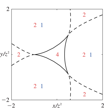
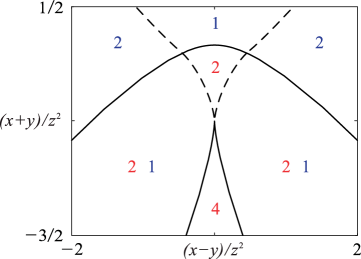
… ►where $j$ denotes a real critical point (36.4.1) or (36.4.2), and $\mu$ denotes a critical point with complex $t$ or $s,t$, connected with $j$ by a steepest-descent path (that is, a path where $\mathrm{\Re }\mathrm{\Phi }=\mathrm{constant}$) in complex $t$ or $(s,t)$ space. … ►

36.5.4 $$80x^5-40x^4-55x^3+5x^2+20x-1=0,$$

ⓘ

Symbols:

$x$: real parameter

Permalink:

http://dlmf.nist.gov/36.5.E4

Encodings:

pMML, png, TeX

See also:

Annotations for §36.5(ii), §36.5(ii), §36.5 and Ch.36

… ►

36.5.7 $$X=\frac{9}{20}+20u^4-\frac{Y^2}{20u^2}+6u^2\mathrm{sign}\left(z\right),$$

ⓘ

Symbols:

$\mathrm{sign}x$: sign of, $z$: real parameter, $X$: scaled coordinate and $Y$: scaled coordinate

Permalink:

http://dlmf.nist.gov/36.5.E7

Encodings:

pMML, png, TeX

See also:

Annotations for §36.5(ii), §36.5(ii), §36.5 and Ch.36

… ►

►►

Figure 36.5.5: Elliptic umbilic catastrophe with $z=\mathrm{constant}$. … Magnify

►

►►

Figure 36.5.6: Hyperbolic umbilic catastrophe with $z=\mathrm{constant}$. Magnify

…

10: 8.26 Tables

… ►

Khamis (1965) tabulates $P(a,x)$ for $a=0.05(.05)10(.1)20(.25)70$, $0.0001\le x\le 250$ to 10D.

… ►

Zhang and Jin (1996, Table 3.8) tabulates $\gamma (a,x)$ for $a=0.5,1,3,5,10,25,50,100$, $x=0(.1)1(1)3,5(5)30,50,100$ to 8D or 8S.

… ►

Abramowitz and Stegun (1964, pp. 245–248) tabulates $E_n\left(x\right)$ for $n=2,3,4,10,20$, $x=0(.01)2$ to 7D; also $(x+n){\mathrm{e}}^x{E}_n\left(x\right)$ for $n=2,3,4,10,20$, $x^{-1}=0(.01)0.1(.05)0.5$ to 6S.

… ►

Pagurova (1961) tabulates $E_n\left(x\right)$ for $n=0(1)20$, $x=0(.01)2(.1)10$ to 4-9S; ${\mathrm{e}}^x{E}_n\left(x\right)$ for $n=2(1)10$, $x=10(.1)20$ to 7D; ${\mathrm{e}}^x{E}_p\left(x\right)$ for $p=0(.1)1$, $x=0.01(.01)7(.05)12(.1)20$ to 7S or 7D.

… ►

Zhang and Jin (1996, Table 19.1) tabulates $E_n\left(x\right)$ for $n=1,2,3,5,10,15,20$, $x=0(.1)1,1.5,2,3,5,10,20,30,50,100$ to 7D or 8S.