…
►Cycles of length one are fixed points.
…
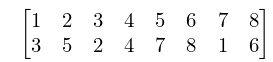
►An element of with fixed points, cycles of length cycles of length , where , is said to have cycle type
.
…
►A derangement is a permutation with no fixed points.
The derangement number, , is the number of elements of with no fixed points:
…
…
►Let be a point set with a limit point
.
As in
…
►If is a finite limit point of , then
…
►Similarly for finite limit point
in place of .
…
►where is a finite, or infinite, limit point of .
…
…
►For applications of Whittaker functions to the uniform asymptotic theory of differential equations with a coalescing turning point and simple pole see §§2.8(vi) and 18.15(i).
…
…
►For applications of the complementary error function in uniform asymptotic approximations of integrals—saddle point coalescing with a pole or saddle point coalescing with an endpoint—see Wong (1989, Chapter 7), Olver (1997b, Chapter 9), and van der Waerden (1951).
…
►Let be any point on the projected spiral.
…
…
►Consider the set of points in that satisfy the equation
…Equation (21.7.1) determines a plane algebraic curve in , which is made compact by adding its points at infinity.
…This compact curve may have singular points, that is, points at which the gradient of vanishes.
…
►The zeros , of specify the finite branch points
, that is, points at which , on the Riemann surface.
Denote the set of all branch points by .
…
…
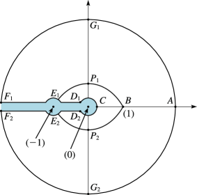
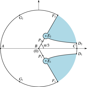
►Corresponding points of the mapping are shown in Figures 10.20.1 and 10.20.2.
…
►The points
where these curves intersect the imaginary axis are , where
…
►►►Figure 10.20.1:
-plane.
and are the points
.
…
Magnify►►►Figure 10.20.2:
-plane.
and are the pointsMagnify
…
…
►Figures 10.41.1 and 10.41.2 show corresponding points of the mapping of the -plane and the -plane.
…Thus is the point
, where is given by (10.20.18).
…
F. W. J. Olver (1976)Improved error bounds for second-order differential equations with two turning points.
J. Res. Nat. Bur. Standards Sect. B80B (4), pp. 437–440.
…
►For discussions of turning points, transition points, and uniform asymptotic expansions for solutions of linear difference equations of the second order see Wang and Wong (2003, 2005).
…
 ►
►
 ►
►
