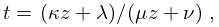
►where , , , are real or complex constants such that .
These constants can be chosen to map any two sets of three distinct points and onto each other.
…
§20.12(ii) Uniformization and Embedding of Complex Tori
►For the terminology and notation see McKean and Moll (1999, pp. 48–53).
►The space of complex tori (that is, the set of complex numbers in which two of these numbers and are regarded as equivalent if there exist integers such that ) is mapped into the projective space via the identification .
Thus theta functions “uniformize” the complex torus.
This ability to uniformize multiply-connected spaces (manifolds), or multi-sheeted functions of a complexvariable (Riemann (1899), Rauch and Lebowitz (1973), Siegel (1988)) has led to applications in string theory (Green et al. (1988a, b), Krichever and Novikov (1989)), and also in statistical mechanics (Baxter (1982)).
…
…
►and assume that the line segment with endpoints and lies in for .
…
►The only cases of that are integrals of the first kind are the two ( or 4) with .
…
►The reduction of is carried out by a relation derived from partial fractions and by use of two recurrence relations.
…
►It depends primarily on multivariate recurrence relations that replace one integral by two or more.
…
►If both square roots in (19.29.22) are 0, then the indeterminacy in the two preceding equations can be removed by using (19.27.8) to evaluate the integral as multiplied either by or by in the cases of (19.29.20) or (19.29.21), respectively.
…
…
►In particular, the principal branch of is defined in a similar way: it corresponds to the principal value of , is analytic in , and two-valued and discontinuous on the cut .
…
►
…
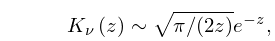
►It has a branch point at for all .
The principal branch corresponds to the principal value of the square root in (10.25.3), is analytic in , and two-valued and discontinuous on the cut .
…
…
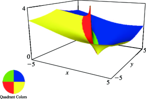
►Because the -function is homogeneous, there is no loss of generality in giving one variable the value or (as in Figure 19.3.2).
For , , and , which are symmetric in , we may further assume that is the largest of if the variables are real, then choose , and consider only and .
…
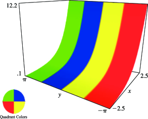
►To view and for complex
, put , use (19.25.1), and see Figures 19.3.7–19.3.12.
…
►To view and for complex
, put , use (19.25.1), and see Figures 19.3.7–19.3.12.
…
 ►
►
 ►
►
