modular equations

SearchAdvancedHelp

(0.001 seconds)

11—20 of 25 matching pages

11: 20.7 Identities

… ►Addendum: For a companion equation see (20.7.34). … ►In the following equations ${\tau }^{\prime }=-1/\tau$, and all square roots assume their principal values. … ►

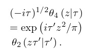
20.7.33 $${(-\mathrm{i}\tau )}^{1/2}{\theta }_4\left(z\right|\tau )=\exp \left(\mathrm{i}{\tau }^{\prime }{z}^2/\pi \right){\theta }_2\left(z{\tau }^{\prime }\right|{\tau }^{\prime }).$$

ⓘ

Symbols:

${\theta }_j\left(z\right|\tau )$: theta function, $\pi$: the ratio of the circumference of a circle to its diameter, $\exp z$: exponential function, $\mathrm{i}$: imaginary unit, $z$: complex and $\tau$: lattice parameter

Referenced by:

(20.10.3), §20.13

Permalink:

http://dlmf.nist.gov/20.7.E33

Encodings:

pMML, png, TeX

See also:

Annotations for §20.7(viii), §20.7 and Ch.20

►These are specific examples of modular transformations as discussed in §23.15; the corresponding results for the general case are given by Rademacher (1973, pp. 181–183). … ►

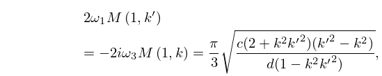
20.7.34 $$\frac{{\theta }_1(z,q^2){\theta }_3(z,q^2)}{{\theta }_1(z,\mathrm{i}q)}=\frac{{\theta }_2(z,q^2){\theta }_4(z,q^2)}{{\theta }_2(z,\mathrm{i}q)}={\mathrm{i}}^{-1/4}\sqrt{\frac{{\theta }_2(0,q^2){\theta }_4(0,q^2)}{2}}.$$

ⓘ

Symbols:

${\theta }_j(z,q)$: theta function, $\mathrm{i}$: imaginary unit, $z$: complex and $q$: nome

Referenced by:

§20.7(iv), Erratum (V1.0.5) for Chapters 8, 20, 36

Permalink:

http://dlmf.nist.gov/20.7.E34

Encodings:

pMML, png, TeX

Addition (effective with 1.0.5):

This equation has been added. See Walker (2012).

See also:

Annotations for §20.7(ix), §20.7 and Ch.20

…

12: Software Index

… ► ►►►►

	Open Source													With Book						Commercial
…
23 Weierstrass Elliptic and Modular Functions
…
28 Mathieu Functions and Hill’s Equation
…

…

13: 27.12 Asymptotic Formulas: Primes

… ►

27.12.5 $$\left|\pi \left(x\right)-\mathrm{li}\left(x\right)\right|=O\left(x\exp \left(-c{(\ln x)}^{1/2}\right)\right),$$ $x\to \mathrm{\infty }$.

ⓘ

Symbols:

$O\left(x\right)$: order not exceeding, $\exp z$: exponential function, $\mathrm{li}\left(x\right)$: logarithmic integral, $\ln z$: principal branch of logarithm function, $\pi \left(x\right)$: number of primes not exceeding a number and $x$: real number

Referenced by:

Erratum (V1.0.18) for Equation (27.12.5)

Permalink:

http://dlmf.nist.gov/27.12.E5

Encodings:

pMML, png, TeX

Change of Notation (effective with 1.0.18):

Replaced $\sqrt{\ln x}$ with ${(\ln x)}^{1/2}$ to be consistent with other equations in this section.

Change of Notation (effective with 1.0.10):

The notation for logarithm has been changed to $\ln$ from $\log$.

See also:

Annotations for §27.12, §27.12 and Ch.27

… ►

27.12.8 $$\frac{\mathrm{li}\left(x\right)}{\varphi \left(m\right)}+O\left(x\exp \left(-\lambda (\alpha ){(\ln x)}^{1/2}\right)\right),$$ $m\le {(\ln x)}^{\alpha }$, $\alpha >0$,

ⓘ

Symbols:

$O\left(x\right)$: order not exceeding, $\varphi \left(n\right)$: Euler’s totient, $\exp z$: exponential function, $\mathrm{li}\left(x\right)$: logarithmic integral, $\ln z$: principal branch of logarithm function, $m$: positive integer and $x$: real number

Referenced by:

Erratum (V1.0.17) for Equation (27.12.8)

Permalink:

http://dlmf.nist.gov/27.12.E8

Encodings:

pMML, png, TeX

Errata (effective with 1.0.17):

Originally the first term was given incorrectly by $\frac{x}{\varphi \left(m\right)}$.

Reported 2017-12-04 by Gergő Nemes

Change of Notation (effective with 1.0.10):

The notation for logarithm has been changed to $\ln$ from $\log$.

See also:

Annotations for §27.12, §27.12 and Ch.27

… ►For example, if $2^n\cancel{\equiv }2(modn)$, then $n$ is composite. … ►A Carmichael number is a composite number $n$ for which $b^n\equiv b(modn)$ for all $b\in \mathbb{N}$. …

14: Bibliography V

… ►

Modular hypergeometric residue sums of elliptic Selberg integrals. Lett. Math. Phys. 58 (3), pp. 223–238.

ⓘ

External Links:

ISSN 0377-9017, Document, MathReview (Laurent Habsieger), ZentralBlatt

Referenced by:

§19.35(i).

Encodings:

BibTeX

… ►

On the coefficients of the modular invariant $J(\tau )$ . Nederl. Akad. Wetensch. Proc. Ser. A. 56 = Indagationes Math. 15 56, pp. 389–400.

ⓘ

External Links:

MathReview (J. Lehner), ZentralBlatt

Referenced by:

§23.17(ii).

Encodings:

BibTeX

… ►

A Mathieu equation for ships rolling among waves. I, II. Norske Vid. Selsk. Forh., Trondheim 22 (25–26), pp. 113–123.

ⓘ

External Links:

MathReview (J. V. Wehausen), ZentralBlatt

Referenced by:

2nd item.

Encodings:

BibTeX

… ►

On the growth of convergence radii for the eigenvalues of the Mathieu equation. Math. Nachr. 192, pp. 239–253.

ⓘ

External Links:

ISSN 0025-584X, Document, MathReview (M. E. Muldoon), ZentralBlatt

Referenced by:

§28.6(i).

Encodings:

BibTeX

… ►

On the rational solutions of the second Painlevé equation. Differ. Uravn. 1 (1), pp. 79–81 (Russian).

ⓘ

Notes:

In Russian. English translation: Differential Equations 1(1), pp. 58–59.

External Links:

MathReview, ZentralBlatt

Referenced by:

§32.8(ii).

Encodings:

BibTeX

…

15: Bibliography C

… ►

Théorie Générale de L’Équation de Mathieu et de quelques autres Équations différentielles de la mécanique. Masson et Cie, Paris (French).

ⓘ

External Links:

MathReview (A. Erdélyi), ZentralBlatt

Referenced by:

§28.1, Notations C, Notations I, Notations I, Notations J, Notations J, Notations S.

Encodings:

BibTeX

… ►

Elementary Differential Equations. Clarendon Press, Oxford.

ⓘ

External Links:

ISBN 0-19-853139-7, MathReview, ZentralBlatt

Referenced by:

§16.12.

Encodings:

BibTeX

… ►

The fourth Painlevé equation and associated special polynomials. J. Math. Phys. 44 (11), pp. 5350–5374.

ⓘ

External Links:

ISSN 0022-2488, Document, MathReview, ZentralBlatt

Referenced by:

§32.8(iv).

Encodings:

BibTeX

… ►

Modular Forms and Fermat’s Last Theorem. Springer-Verlag, New York.

ⓘ

External Links:

ISBN 0-387-94609-8; 0-387-98998-6, MathReview (M. Ram Murty), ZentralBlatt

Referenced by:

§23.20(v).

Encodings:

BibTeX

… ►

Algorithms for Modular Elliptic Curves. 2nd edition, Cambridge University Press, Cambridge.

ⓘ

External Links:

ISBN 0-521-59820-6, MathReview (Joseph H. Silverman), ZentralBlatt

Referenced by:

§23.20(ii).

Encodings:

BibTeX

…

16: Mathematical Introduction

… ►These include, for example, multivalued functions of complex variables, for which new definitions of branch points and principal values are supplied (§§1.10(vi), 4.2(i)); the Dirac delta (or delta function), which is introduced in a more readily comprehensible way for mathematicians (§1.17); numerically satisfactory solutions of differential and difference equations (§§2.7(iv), 2.9(i)); and numerical analysis for complex variables (Chapter 3). … ►This is because $𝐅$ is akin to the notation used for Bessel functions (§10.2(ii)), inasmuch as $𝐅$ is an entire function of each of its parameters $a$, $b$, and $c$:​ this results in fewer restrictions and simpler equations. … ► ►►►

$(a,b]$ or $[a,b)$	half-closed intervals.
…
$mod$ or modulo	$m\equiv n(modp)$ means $p$ divides $m-n$, where $m$, $n$, and $p$ are positive integers with $m>n$.
…

… ►For all equations and other technical information this Handbook and the DLMF either provide references to the literature for proof or describe steps that can be followed to construct a proof. … ►For equations or other technical information that appeared previously in AMS 55, the DLMF usually includes the corresponding AMS 55 equation number, or other form of reference, together with corrections, if needed. …

17: Bibliography K

… ►

Asymptotic behavior of the solutions of the Painlevé equation of the first kind. Differ. Uravn. 24 (10), pp. 1684–1695 (Russian).

ⓘ

Notes:

In Russian. English translation: Differential Equations 24(1988), no. 10, pp. 1107–1115 (1989)

External Links:

ISSN 0374-0641, MathReview, ZentralBlatt

Referenced by:

§32.11(i).

Encodings:

BibTeX

… ►

Rational solutions of the fifth Painlevé equation. Differential Integral Equations 7 (3-4), pp. 967–1000.

ⓘ

External Links:

ISSN 0893-4983, MathReview, ZentralBlatt

Referenced by:

§32.8(v).

Encodings:

BibTeX

… ►

Introduction to Elliptic Curves and Modular Forms. 2nd edition, Graduate Texts in Mathematics, Vol. 97, Springer-Verlag, New York.

ⓘ

External Links:

ISBN 0-387-97966-2, MathReview, ZentralBlatt

Referenced by:

§20.10(i), §20.12(i), §20.9(iii), §22.18(iv), §23.1, §23.20(ii), §23.20(v), Ch.23.

Encodings:

BibTeX

… ►

Asymptotic solution of Maxwell’s equations near caustics. Izv. Vuz. Radiofiz. 7, pp. 1049–1056.

ⓘ

Referenced by:

§36.14(i).

Encodings:

BibTeX

… ►

The Korteweg-de Vries Equation and Related Evolution Equations. In Nonlinear Wave Motion (Proc. AMS-SIAM Summer Sem., Clarkson Coll. Tech., Potsdam, N.Y., 1972), A. C. Newell (Ed.), Lectures in Appl. Math., Vol. 15, pp. 61–83.

ⓘ

External Links:

MathReview (G. L. Lamb, Jr.), ZentralBlatt

Referenced by:

§22.19(iii).

Encodings:

BibTeX

…

18: Errata

… ►

Equation (16.16.5_5).

… ►

These equations, originally added in Other Changes and Other Changes, respectively, have been assigned interpolated numbers.

… ►

Four of the terms were rewritten for improved clarity.

… ►

has been generalized to cover an additional case.

… ►

These equations have been rewritten to improve the numerical computation of $\arctan x$.

…

19: 23.22 Methods of Computation

… ►The modular functions $\lambda \left(\tau \right)$, $J\left(\tau \right)$, and $\eta \left(\tau \right)$ are also obtainable in a similar manner from their definitions in §23.15(ii). … ►Suppose that the invariants $g_2=c$, $g_3=d$, are given, for example in the differential equation (23.3.10) or via coefficients of an elliptic curve (§23.20(ii)). … ►

In the general case, given by $cd\ne 0$, we compute the roots $\alpha$, $\beta$, $\gamma$, say, of the cubic equation $4t^3-ct-d=0$; see §1.11(iii). These roots are necessarily distinct and represent $e_1$, $e_2$, $e_3$ in some order.

If $c$ and $d$ are real, and the discriminant is positive, that is $c^3-27d^2>0$, then $e_1$, $e_2$, $e_3$ can be identified via (23.5.1), and $k^2$, $k_{}^{\prime }{}_{}{}^2$ obtained from (23.6.16).

If , or $c$ and $d$ are not both real, then we label $\alpha$, $\beta$, $\gamma$ so that the triangle with vertices $\alpha$, $\beta$, $\gamma$ is positively oriented and $[\alpha ,\gamma ]$ is its longest side (chosen arbitrarily if there is more than one). In particular, if $\alpha$, $\beta$, $\gamma$ are collinear, then we label them so that $\beta$ is on the line segment $(\alpha ,\gamma )$. In consequence, $k^2=(\beta -\gamma )/(\alpha -\gamma )$, $k_{}^{\prime }{}_{}{}^2=(\alpha -\beta )/(\alpha -\gamma )$ satisfy $\mathrm{\Im }{k}^2\ge 0\ge \mathrm{\Im }k_{}^{\prime }{}_{}{}^2$ (with strict inequality unless $\alpha$, $\beta$, $\gamma$ are collinear); also $|k^2|$, $|k_{}^{\prime }{}_{}{}^2|\le 1$.

Finally, on taking the principal square roots of $k^2$ and $k_{}^{\prime }{}_{}{}^2$ we obtain values for $k$ and $k^{\prime }$ that lie in the 1st and 4th quadrants, respectively, and $2{\omega }_1$, $2{\omega }_3$ are given by

23.22.1 $$2{\omega }_{1}M(1,k^{\prime })=-2\mathrm{i}{\omega }_{3}M(1,k)=\frac{\pi }{3}\sqrt{\frac{c(2+k^{2}k_{}^{\prime }{}_{}{}^2)(k_{}^{\prime }{}_{}{}^2-k^2)}{d(1-k^{2}k_{}^{\prime }{}_{}{}^2)}},$$

ⓘ

Symbols:

$M(a,g)$: arithmetic-geometric mean, $\pi$: the ratio of the circumference of a circle to its diameter, $\mathrm{i}$: imaginary unit, ${\omega }_1$, ${\omega }_3$, ${\omega }_2=-{\omega }_1-{\omega }_3$: lattice generators, $k$: modulus and $k^{\prime }$: complementary modulus

Proof sketch:

Combine (23.6.16), (23.6.17), (22.20.6), (23.3.5)–(23.3.7), and use analytical continuation.

Referenced by:

§23.22(ii)

Permalink:

http://dlmf.nist.gov/23.22.E1

Encodings:

pMML, png, TeX

See also:

Annotations for §23.22(ii), §23.22(ii), §23.22 and Ch.23

where $M$ denotes the arithmetic-geometric mean (see §§19.8(i) and 22.20(ii)). This process yields 2 possible pairs ($2{\omega }_1$, $2{\omega }_3$), corresponding to the 2 possible choices of the square root.

…

20: 24.19 Methods of Computation

… ►Equations (24.5.3) and (24.5.4) enable $B_n$ and $E_n$ to be computed by recurrence. … ►For number-theoretic applications it is important to compute $B_{2n}(modp)$ for $2n\le p-3$; in particular to find the irregular pairs $(2n,p)$ for which $B_{2n}\equiv 0(modp)$. …