maximum modulus
(0.001 seconds)
21—30 of 47 matching pages
21: 2.5 Mellin Transform Methods
…
►Let and .
…In the half-plane , the product has a pole of order two at each positive integer, and
…
►We now apply (2.5.5) with , and then translate the integration contour to the right.
…
►From (2.5.26) and (2.5.28), it follows that both and are defined in the half-plane .
…
►Put and break the integration range at , as in (2.5.23) and (2.5.24).
…
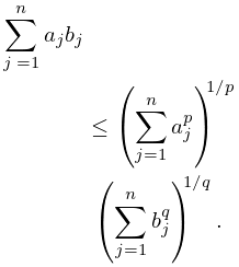
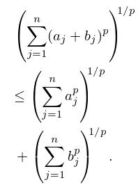
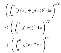
22: 1.7 Inequalities
23: 2.11 Remainder Terms; Stokes Phenomenon
…
►In both the modulus and phase of the asymptotic variable need to be taken into account.
…
►In the transition through , changes very rapidly, but smoothly, from one form to the other; compare the graph of its modulus in Figure 2.11.1 in the case .
…
►Rays (or curves) on which one contribution in a compound asymptotic expansion achieves maximum dominance over another are called Stokes lines ( in the present example).
…
►(This means that, if necessary, is replaced by .)
…
►The process just used is equivalent to re-expanding the remainder term of the original asymptotic series (2.11.24) in powers of and truncating the new series optimally.
…
24: Bibliography L
…
►
A partition function connected with the modulus five.
Duke Math. J. 8 (4), pp. 631–655.
…
►
Optimal cylindrical and spherical Bessel transforms satisfying bound state boundary conditions.
Comput. Phys. Comm. 99 (2-3), pp. 297–306.
…
►
Algorithm 344: Student’s t-distribution [S14].
Comm. ACM 12 (1), pp. 37–38.
…
►
Algorithm 244: Fresnel integrals.
Comm. ACM 7 (11), pp. 660–661.
…
25: 22.20 Methods of Computation
…
►A powerful way of computing the twelve Jacobian elliptic functions for real or complex values of both the argument and the modulus
is to use the definitions in terms of theta functions given in §22.2, obtaining the theta functions via methods described in §20.14.
…
►Given real or complex numbers , with not real and negative, define
…
►From (22.7.1), and .
…
►If either or is given, then we use , , , and , obtaining the values of the theta functions as in §20.14.
…
►If , then three iterations of (22.20.1) give , and from (22.20.6) — in agreement with the value of ; compare (23.17.3) and (23.22.2).
…
26: Bibliography W
…
►
Algorithm 794: Numerical Hankel transform by the Fortran program HANKEL.
ACM Trans. Math. Software 25 (2), pp. 240–250.
…
►
Some explicit Padé approximants for the function and a related quadrature formula involving Bessel functions.
SIAM J. Math. Anal. 16 (4), pp. 887–895.
…
►
Algorithm 44: Bessel functions computed recursively.
Comm. ACM 4 (4), pp. 177–178.
…
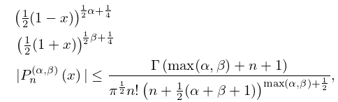
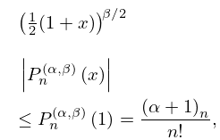
27: 18.14 Inequalities
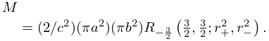
28: 19.34 Mutual Inductance of Coaxial Circles
…
►
19.34.1
…
►is the square of the maximum (upper signs) or minimum (lower signs) distance between the circles.
…
►
19.34.7
…
29: Bibliography S
…
►
Parabolic cylinder functions of integer and half-integer orders for nonnegative arguments.
Comput. Phys. Comm. 115 (1), pp. 69–86.
…
►
Algorithm 723: Fresnel integrals.
ACM Trans. Math. Software 19 (4), pp. 452–456.
…
►
On numerical Bessel transformation.
Comput. Phys. Comm. 16 (3), pp. 383–387.
…
►
Automatic computing methods for special functions. I.
J. Res. Nat. Bur. Standards Sect. B 74B, pp. 211–224.
…
►
Root-rational-fraction package for exact calculation of vector-coupling coefficients.
Comput. Phys. Comm. 21 (2), pp. 195–205.
…
