locally%20integrable

SearchAdvancedHelp

(0.001 seconds)

11—20 of 358 matching pages

11: 18.39 Applications in the Physical Sciences

… ►These eigenfunctions are quantum wave-functions whose absolute values squared give the probability density of finding the single particle at hand at position $x$ in the $n$th eigenstate, namely that probability is $P(x\to x+\mathrm{\Delta }x)$ = ${|{\psi }_n(x)|}^2\mathrm{\Delta }(x)$, $\mathrm{\Delta }(x)$ being a localized interval on the $x$-axis. … ►with an infinite set of orthonormal $L^2$ eigenfunctions … ►Derivations of (18.39.42) appear in Bethe and Salpeter (1957, pp. 12–20), and Pauling and Wilson (1985, Chapter V and Appendix VII), where the derivations are based on (18.39.36), and is also the notation of Piela (2014, §4.7), typifying the common use of the associated Coulomb–Laguerre polynomials in theoretical quantum chemistry. … ►The bound state $L^2$ eigenfunctions of the radial Coulomb Schrödinger operator are discussed in §§18.39(i) and 18.39(ii), and the $\delta$-function normalized (non-$L^2$) in Chapter 33, where the solutions appear as Whittaker functions. … ►The fact that non-$L^2$ continuum scattering eigenstates may be expressed in terms or (infinite) sums of $L^2$ functions allows a reformulation of scattering theory in atomic physics wherein no non-$L^2$ functions need appear. …

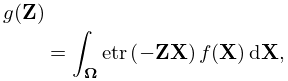
12: 35.2 Laplace Transform

… ►

35.2.1 $$g(𝐙)={\int }_{𝛀}\mathrm{etr}\left(-𝐙𝐗\right)f(𝐗)d𝐗,$$

ⓘ

Defines:

$g$: Laplace transformation of $f$ (locally)

Symbols:

$\mathrm{etr}\left(𝐀\right)$: exponential of trace, $\int$: integral, $𝐗$: real symmetric $m\times m$ matrix, $d$: differential of matrix, $𝛀$: space of positive-definite real symmetric $m\times m$ matrices, $𝐙$: complex symmetric $m\times m$ matrix and $f(𝐗)$: complex-valued function of matrix argument

Keywords:

Laplace transform

Referenced by:

§35.2

Permalink:

http://dlmf.nist.gov/35.2.E1

Encodings:

pMML, png, TeX

See also:

Annotations for §35.2, §35.2 and Ch.35

►where the integration variable $𝐗$ ranges over the space $𝛀$. … ►

35.2.3

ⓘ

Defines:

$\ast$: convolution operator (locally)

Symbols:

$\int$: integral, $𝐓$: real symmetric $m\times m$ matrix, $𝐗$: real symmetric $m\times m$ matrix, $d$: differential of matrix, : less-than for matrices, $f(𝐗)$: complex-valued function of matrix argument and $𝟎$: $m\times m$ matrix of zeros

Referenced by:

§35.6(ii)

Permalink:

http://dlmf.nist.gov/35.2.E3

Encodings:

pMML, png, TeX

See also:

Annotations for §35.2, §35.2 and Ch.35

13: 1.4 Calculus of One Variable

… ►

Maxima and Minima

… ►

§1.4(iv) Indefinite Integrals

… ►

Integration by Parts

… ►

§1.4(v) Definite Integrals

… ►

Square-Integrable Functions

…

14: 3.7 Ordinary Differential Equations

… ►

3.7.1 $$\frac{d^{2}w}{{dz}^2}+f(z)\frac{dw}{dz}+g(z)w=h(z),$$

ⓘ

Defines:

$f(z)$: function (locally), $g(z)$: function (locally) and $h(z)$: function (locally)

Symbols:

$\frac{df}{dx}$: derivative of $f$ with respect to $x$ and $w(z)$: function

Referenced by:

§3.7(i), §3.7(ii), §3.7(ii), §3.7(ii)

Permalink:

http://dlmf.nist.gov/3.7.E1

Encodings:

pMML, png, TeX

See also:

Annotations for §3.7(i), §3.7 and Ch.3

… ►Assume that we wish to integrate (3.7.1) along a finite path $𝒫$ from $z=a$ to $z=b$ in a domain $D$. … ►

3.7.6

ⓘ

Defines:

$𝐀(\tau ,z)$: matrix (locally) and $A_{jk}(\tau ,z)$: matrix entry (locally)

Permalink:

http://dlmf.nist.gov/3.7.E6

Encodings:

pMML, png, TeX

See also:

Annotations for §3.7(ii), §3.7 and Ch.3

… ►

3.7.7 $$𝐛(\tau ,z)=\left[\begin{array}{c}{b}_1(\tau ,z)\\ b_2(\tau ,z)\end{array}\right],$$

ⓘ

Defines:

$𝐛(\tau ,z)$: vector (locally) and $b_j(\tau ,z)$: vector (locally)

Permalink:

http://dlmf.nist.gov/3.7.E7

Encodings:

pMML, png, TeX

See also:

Annotations for §3.7(ii), §3.7 and Ch.3

… ►The larger the absolute values of the eigenvalues ${\lambda }_k$ that are being sought, the smaller the integration steps $\left|{\tau }_j\right|$ need to be. …

15: 4.42 Solution of Triangles

…

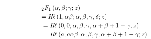
16: 31.7 Relations to Other Functions

… ►

31.7.1 $${}_2{}^{}F_1^{}(\alpha ,\beta ;\gamma ;z)=H\mathrm{\ell }(1,\alpha \beta ;\alpha ,\beta ,\gamma ,\delta ;z)=H\mathrm{\ell }(0,0;\alpha ,\beta ,\gamma ,\alpha +\beta +1-\gamma ;z)=H\mathrm{\ell }(a,a\alpha \beta ;\alpha ,\beta ,\gamma ,\alpha +\beta +1-\gamma ;z).$$

ⓘ

Symbols:

${}_2{}^{}F_1^{}(a,b;c;z)$: $=F(a,b;c;z)$ notation for Gauss’ hypergeometric function, $H\mathrm{\ell }(a,q;\alpha ,\beta ,\gamma ,\delta ;z)$: Heun functions, $z$: complex variable, $\gamma$: real or complex parameter, $\delta$: real or complex parameter, $a$: complex parameter, $\alpha$: real or complex parameter and $\beta$: real or complex parameter

Permalink:

http://dlmf.nist.gov/31.7.E1

Encodings:

pMML, png, TeX

See also:

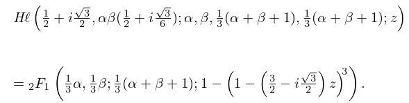
Annotations for §31.7(i), §31.7 and Ch.31

►Other reductions of $H\mathrm{\ell }$ to a ${}_2{}^{}F_1^{}$, with at least one free parameter, exist iff the pair $(a,p)$ takes one of a finite number of values, where $q=\alpha \beta p$. … ►

31.7.2 $$H\mathrm{\ell }(2,\alpha \beta ;\alpha ,\beta ,\gamma ,\alpha +\beta -2\gamma +1;z)={}_2{}^{}F_1^{}(\frac{1}{2}\alpha ,\frac{1}{2}\beta ;\gamma ;1-{(1-z)}^2),$$

ⓘ

Symbols:

${}_2{}^{}F_1^{}(a,b;c;z)$: $=F(a,b;c;z)$ notation for Gauss’ hypergeometric function, $H\mathrm{\ell }(a,q;\alpha ,\beta ,\gamma ,\delta ;z)$: Heun functions, $z$: complex variable, $\gamma$: real or complex parameter, $\alpha$: real or complex parameter and $\beta$: real or complex parameter

Permalink:

http://dlmf.nist.gov/31.7.E2

Encodings:

pMML, png, TeX

See also:

Annotations for §31.7(i), §31.7 and Ch.31

►

31.7.3 $$H\mathrm{\ell }(4,\alpha \beta ;\alpha ,\beta ,\frac{1}{2},\frac{2}{3}(\alpha +\beta );z)={}_2{}^{}F_1^{}(\frac{1}{3}\alpha ,\frac{1}{3}\beta ;\frac{1}{2};1-{(1-z)}^2(1-\frac{1}{4}z)),$$

ⓘ

Symbols:

${}_2{}^{}F_1^{}(a,b;c;z)$: $=F(a,b;c;z)$ notation for Gauss’ hypergeometric function, $H\mathrm{\ell }(a,q;\alpha ,\beta ,\gamma ,\delta ;z)$: Heun functions, $z$: complex variable, $\alpha$: real or complex parameter and $\beta$: real or complex parameter

Permalink:

http://dlmf.nist.gov/31.7.E3

Encodings:

pMML, png, TeX

See also:

Annotations for §31.7(i), §31.7 and Ch.31

►

31.7.4 $$H\mathrm{\ell }(\frac{1}{2}+\mathrm{i}\frac{\sqrt{3}}{2},\alpha \beta (\frac{1}{2}+\mathrm{i}\frac{\sqrt{3}}{6});\alpha ,\beta ,\frac{1}{3}(\alpha +\beta +1),\frac{1}{3}(\alpha +\beta +1);z)={}_2{}^{}F_1^{}(\frac{1}{3}\alpha ,\frac{1}{3}\beta ;\frac{1}{3}(\alpha +\beta +1);1-{\left(1-\left(\frac{3}{2}-\mathrm{i}\frac{\sqrt{3}}{2}\right)z\right)}^3).$$

ⓘ

Symbols:

${}_2{}^{}F_1^{}(a,b;c;z)$: $=F(a,b;c;z)$ notation for Gauss’ hypergeometric function, $H\mathrm{\ell }(a,q;\alpha ,\beta ,\gamma ,\delta ;z)$: Heun functions, $\mathrm{i}$: imaginary unit, $z$: complex variable, $\alpha$: real or complex parameter and $\beta$: real or complex parameter

Permalink:

http://dlmf.nist.gov/31.7.E4

Encodings:

pMML, png, TeX

See also:

Annotations for §31.7(i), §31.7 and Ch.31

…

17: 36.5 Stokes Sets

… ►

36.5.4 $$80x^5-40x^4-55x^3+5x^2+20x-1=0,$$

ⓘ

Symbols:

$x$: real parameter

Permalink:

http://dlmf.nist.gov/36.5.E4

Encodings:

pMML, png, TeX

See also:

Annotations for §36.5(ii), §36.5(ii), §36.5 and Ch.36

… ►

36.5.7 $$X=\frac{9}{20}+20u^4-\frac{Y^2}{20u^2}+6u^2\mathrm{sign}\left(z\right),$$

ⓘ

Symbols:

$\mathrm{sign}x$: sign of, $z$: real parameter, $X$: scaled coordinate and $Y$: scaled coordinate

Permalink:

http://dlmf.nist.gov/36.5.E7

Encodings:

pMML, png, TeX

See also:

Annotations for §36.5(ii), §36.5(ii), §36.5 and Ch.36

… ►

36.5.13 $$w=u-\frac{2}{3}+{\left({\left(\frac{2}{3}-u\right)}^2+\left|\frac{y}{6z^2}\right|{\left(\frac{\frac{2}{3}-u}{u}\right)}^{1/2}\right)}^{1/2},$$

ⓘ

Defines:

$w$: quantity (locally)

Symbols:

$y$: real parameter and $z$: real parameter

Permalink:

http://dlmf.nist.gov/36.5.E13

Encodings:

pMML, png, TeX

See also:

Annotations for §36.5(iii), §36.5(iii), §36.5 and Ch.36

…

18: 9.13 Generalized Airy Functions

… ►

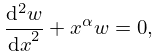
9.13.1 $$\frac{d^{2}w}{{dz}^2}=z^{n}w,$$ $n=1,2,3,\mathrm{\dots }$,

ⓘ

Defines:

$n$: parameter (locally)

Symbols:

$\frac{df}{dx}$: derivative of $f$ with respect to $x$ , $z$: complex variable and $w$: function

Source:

Swanson and Headley (1967, (1))

Referenced by:

§9.13(i), §9.13(i), §9.13(i)

Permalink:

http://dlmf.nist.gov/9.13.E1

Encodings:

pMML, png, TeX

See also:

Annotations for §9.13(i), §9.13 and Ch.9

… ►

9.13.19 $$\frac{d^{2}w}{{dx}^2}+x^{\alpha }w=0,$$

ⓘ

Defines:

$\alpha$: parameter (locally) and $x$: parameter (locally)

Symbols:

$\frac{df}{dx}$: derivative of $f$ with respect to $x$ and $w$: function

Source:

Smirnov (1960, (1.2), p. 1)

Permalink:

http://dlmf.nist.gov/9.13.E19

Encodings:

pMML, png, TeX

See also:

Annotations for §9.13(i), §9.13 and Ch.9

… ►

9.13.25 $$A_k(z,p)=\frac{1}{2\pi \mathrm{i}}{\int }_{{ℒ}_k}{t}^{-p}\exp \left(zt-\frac{1}{3}{t}^3\right)dt,$$ $k=1,2,3$, $p\in ℂ$,

ⓘ

Defines:

$k$: index (locally) and $p$: parameter (locally)

Symbols:

$A_k(z,p)$: generalized Airy function, $\pi$: the ratio of the circumference of a circle to its diameter, $ℂ$: complex plane, $dx$: differential of $x$ , $\in$: element of, $\exp z$: exponential function, $\mathrm{i}$: imaginary unit, $\int$: integral, $z$: complex variable and $ℒ$: integration path

Sources:

Reid (1972, (A4), p. 362); Drazin and Reid (1981, (A4), p. 466)

Referenced by:

§9.13(ii)

Permalink:

http://dlmf.nist.gov/9.13.E25

Encodings:

pMML, png, TeX

See also:

Annotations for §9.13(ii), §9.13 and Ch.9

… ►The integration paths ${ℒ}_0$, ${ℒ}_1$, ${ℒ}_2$, ${ℒ}_3$ are depicted in Figure 9.13.1. … ►

9.13.32 $$f(p-3)-zf(p-1)+(p-1)f(p)=0.$$

ⓘ

Defines:

$f$: function (locally)

Symbols:

$z$: complex variable and $p$: parameter

Source:

Reid (1972, (A9), p. 363)

Permalink:

http://dlmf.nist.gov/9.13.E32

Encodings:

pMML, png, TeX

See also:

Annotations for §9.13(ii), §9.13 and Ch.9

…

19: 12.11 Zeros

… ►

12.11.2 $${\tau }_s=\left(2s+\frac{1}{2}-a\right)\pi +\mathrm{i}\ln \left({\pi }^{-\frac{1}{2}}{2}^{-a-\frac{1}{2}}\mathrm{\Gamma }\left(\frac{1}{2}+a\right)\right),$$

ⓘ

Defines:

${\tau }_s$ (locally)

Symbols:

$\mathrm{\Gamma }\left(z\right)$: gamma function, $\pi$: the ratio of the circumference of a circle to its diameter, $\mathrm{i}$: imaginary unit, $\ln z$: principal branch of logarithm function, $s$: nonnegative integer and $a$: real or complex parameter

Permalink:

http://dlmf.nist.gov/12.11.E2

Encodings:

pMML, png, TeX

See also:

Annotations for §12.11(ii), §12.11 and Ch.12

… ►

12.11.3 $${\lambda }_s=\ln {\tau }_s-\frac{1}{2}\pi \mathrm{i}.$$

ⓘ

Defines:

${\lambda }_s$ (locally)

Symbols:

$\pi$: the ratio of the circumference of a circle to its diameter, $\mathrm{i}$: imaginary unit, $\ln z$: principal branch of logarithm function, $s$: nonnegative integer and ${\tau }_s$

Permalink:

http://dlmf.nist.gov/12.11.E3

Encodings:

pMML, png, TeX

See also:

Annotations for §12.11(ii), §12.11 and Ch.12

… ►

12.11.4 $$u_{a,s}\sim 2^{\frac{1}{2}}\mu \left(p_0(\alpha )+\frac{p_1(\alpha )}{{\mu }^4}+\frac{p_2(\alpha )}{{\mu }^8}+\mathrm{\cdots }\right),$$

ⓘ

Defines:

$u_{a,s}$: zeros (locally)

Symbols:

$\sim$: Poincaré asymptotic expansion, $s$: nonnegative integer, $a$: real or complex parameter, $\alpha$ and $p_n(\zeta )$: coefficients

Referenced by:

§12.11(iii)

Permalink:

http://dlmf.nist.gov/12.11.E4

Encodings:

pMML, png, TeX

See also:

Annotations for §12.11(iii), §12.11 and Ch.12

… ►

12.11.7 $$u_{a,s}^{\prime }\sim 2^{\frac{1}{2}}\mu \left(q_0(\beta )+\frac{q_1(\beta )}{{\mu }^4}+\frac{q_2(\beta )}{{\mu }^8}+\mathrm{\cdots }\right),$$

ⓘ

Defines:

$u_{a,s}^{\prime }$: zeros (locally)

Symbols:

$\sim$: Poincaré asymptotic expansion, $s$: nonnegative integer, $a$: real or complex parameter and $\beta$

Permalink:

http://dlmf.nist.gov/12.11.E7

Encodings:

pMML, png, TeX

See also:

Annotations for §12.11(iii), §12.11 and Ch.12

… ►

12.11.9 $$u_{a,1}\sim 2^{\frac{1}{2}}\mu \left(1-\mathrm{1.85575\hspace{0.33em}708}{\mu }^{-4/3}-\mathrm{0.34438\hspace{0.33em}34}{\mu }^{-8/3}-\mathrm{0.16871\hspace{0.33em}5}{\mu }^{-4}-0.11414{\mu }^{-16/3}-0.0808{\mu }^{-20/3}-\mathrm{\cdots }\right),$$

ⓘ

Symbols:

$\sim$: Poincaré asymptotic expansion, $a$: real or complex parameter and $u_{a,s}$: zeros

Referenced by:

§12.11(iii)

Permalink:

http://dlmf.nist.gov/12.11.E9

Encodings:

pMML, png, TeX

See also:

Annotations for §12.11(iii), §12.11 and Ch.12

…

20: 1.18 Linear Second Order Differential Operators and Eigenfunction Expansions

… ►We integrate by parts twice giving: … ►Eigenfunctions corresponding to the continuous spectrum are non-$L^2$ functions. … ►Should $q(x)$ be bounded but random, leading to Anderson localization, the spectrum could range from being a dense point spectrum to being singular continuous, see Simon (1995), Avron and Simon (1982); a good general reference being Cycon et al. (2008, Ch. 9 and 10). … … ►Thus, and this is a case where $q(x)$ is not continuous, if $q(x)=-\alpha \delta \left(x-a\right)$, $\alpha >0$, there will be an $L^2$ eigenfunction localized in the vicinity of $x=a$, with a negative eigenvalue, thus disjoint from the continuous spectrum on $[0,\mathrm{\infty })$. …