little q-Jacobi polynomials

SearchAdvancedHelp

(0.003 seconds)

21—30 of 271 matching pages

21: 24.18 Physical Applications

§24.18 Physical Applications

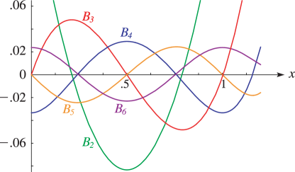
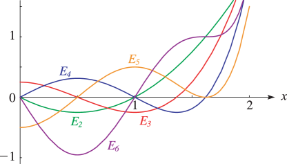
►Bernoulli polynomials appear in statistical physics (Ordóñez and Driebe (1996)), in discussions of Casimir forces (Li et al. (1991)), and in a study of quark-gluon plasma (Meisinger et al. (2002)). ►Euler polynomials also appear in statistical physics as well as in semi-classical approximations to quantum probability distributions (Ballentine and McRae (1998)).

22: 3.2 Linear Algebra

… ►When the factorization (3.2.5) is available, the accuracy of the computed solution $𝐱$ can be improved with little extra computation. … ►The polynomial …The multiplicity of an eigenvalue is its multiplicity as a zero of the characteristic polynomial (§3.8(i)). … … ►Its characteristic polynomial can be obtained from the recursion …

23: Bibliography D

… ►

Computing Riemann matrices of algebraic curves. Phys. D 152/153, pp. 28–46.

ⓘ

External Links:

ISSN 0167-2789, Document, MathReview (John B. Little), ZentralBlatt

Referenced by:

3rd item.

Encodings:

BibTeX

… ►

On the real roots of Euler polynomials. Monatsh. Math. 106 (2), pp. 115–138.

ⓘ

External Links:

ISSN 0026-9255, MathReview (H. M. Srivastava), ZentralBlatt

Referenced by:

§24.12(ii).

Encodings:

BibTeX

… ►

On multiple zeros of Bernoulli polynomials. Acta Arith. 134 (2), pp. 149–155.

ⓘ

External Links:

ISSN 0065-1036, Document, MathReview (Arnold M. Adelberg), ZentralBlatt

Referenced by:

§24.12(iv).

Encodings:

BibTeX

… ►

Orthogonal polynomials and the construction of piecewise polynomial smooth wavelets. SIAM J. Math. Anal. 30 (5), pp. 1029–1056.

ⓘ

External Links:

ISSN 0036-1410, Document, MathReview (Kathi Karima Selig), ZentralBlatt

Referenced by:

§16.4(iii).

Encodings:

BibTeX

… ►

Uniform asymptotic expansions for Charlier polynomials. J. Approx. Theory 112 (1), pp. 93–133.

ⓘ

External Links:

ISSN 0021-9045, Document, MathReview (Eberhard Wagner), ZentralBlatt

Referenced by:

§18.24.

Encodings:

BibTeX

…

24: 27.16 Cryptography

… ►Procedures for finding such primes require very little computer time. …

25: 4.13 Lambert $W$-Function

… ►

4.13.1_1 $$W_k\left(z\right)={\ln }_k(z)-\ln \left({\ln }_k(z)\right)+o\left(1\right),$$ $\left|z\right|\to \mathrm{\infty }$,

ⓘ

Symbols:

$W\left(z\right)$: Lambert $W$-function, $o\left(x\right)$: order less than, $\ln z$: principal branch of logarithm function, $k$: integer and $z$: complex variable

Notes:

See Corless et al. (1996, §4).

Permalink:

http://dlmf.nist.gov/4.13.E1_1

Encodings:

pMML, png, TeX

Addition (effective with 1.1.7):

This equation was added.

See also:

Annotations for §4.13 and Ch.4

… ►in which the $p_n(x)$ are polynomials of degree $n$ with …

26: 24.3 Graphs

… ►

►►

Figure 24.3.1: Bernoulli polynomials $B_n\left(x\right)$, $n=2,3,\mathrm{\dots },6$. Magnify

►

►►

Figure 24.3.2: Euler polynomials $E_n\left(x\right)$, $n=2,3,\mathrm{\dots },6$. Magnify

27: 18.4 Graphics

… ►

►►

Figure 18.4.1: Jacobi polynomials $P_n^{(1.5,-0.5)}\left(x\right)$, $n=1,2,3,4,5$. Magnify

►

►►

Figure 18.4.2: Jacobi polynomials $P_n^{(1.25,0.75)}\left(x\right)$, $n=7,8$. … Magnify

… ►

►►

Figure 18.4.4: Legendre polynomials $P_n\left(x\right)$, $n=1,2,3,4,5$. Magnify

►

►►

Figure 18.4.5: Laguerre polynomials $L_n\left(x\right)$, $n=1,2,3,4,5$. Magnify

… ►

►►

Figure 18.4.7: Monic Hermite polynomials $h_n(x)=2^{-n}{H}_n\left(x\right)$, $n=1,2,3,4,5$. Magnify

…

28: 18.7 Interrelations and Limit Relations

§18.7 Interrelations and Limit Relations

… ►

Chebyshev, Ultraspherical, and Jacobi

… ►

Legendre, Ultraspherical, and Jacobi

… ►

§18.7(ii) Quadratic Transformations

… ►

§18.7(iii) Limit Relations

…

29: 10.7 Limiting Forms

… ►

10.7.6 $$Y_{\mathrm{i}\nu }\left(z\right)=\frac{\mathrm{i}\mathrm{csch}\left(\nu \pi \right)}{\mathrm{\Gamma }\left(1-\mathrm{i}\nu \right)}{(\frac{1}{2}z)}^{-\mathrm{i}\nu }-\frac{\mathrm{i}\coth \left(\nu \pi \right)}{\mathrm{\Gamma }\left(1+\mathrm{i}\nu \right)}{(\frac{1}{2}z)}^{\mathrm{i}\nu }+{\mathrm{e}}^{|\nu \mathrm{ph}z|}o\left(1\right),$$ $\nu \in ℝ$ and $\nu \ne 0$.

ⓘ

Symbols:

$Y_{\nu }\left(z\right)$: Bessel function of the second kind, $\mathrm{\Gamma }\left(z\right)$: gamma function, $\pi$: the ratio of the circumference of a circle to its diameter, $\in$: element of, $\mathrm{e}$: base of natural logarithm, $\mathrm{csch}z$: hyperbolic cosecant function, $\coth z$: hyperbolic cotangent function, $\mathrm{i}$: imaginary unit, $o\left(x\right)$: order less than, $\mathrm{ph}$: phase, $ℝ$: real line, $z$: complex variable and $\nu$: complex parameter

Referenced by:

§10.7(i), §10.7(i)

Permalink:

http://dlmf.nist.gov/10.7.E6

Encodings:

pMML, png, TeX

See also:

Annotations for §10.7(i), §10.7 and Ch.10

… ►

$$J_{\nu }\left(z\right)=\sqrt{2/(\pi z)}\left(\cos \left(z-\frac{1}{2}\nu \pi -\frac{1}{4}\pi \right)+{\mathrm{e}}^{|\mathrm{\Im }z|}o\left(1\right)\right),$$

►

$$Y_{\nu }\left(z\right)=\sqrt{2/(\pi z)}\left(\sin \left(z-\frac{1}{2}\nu \pi -\frac{1}{4}\pi \right)+{\mathrm{e}}^{|\mathrm{\Im }z|}o\left(1\right)\right),$$ .

…

30: 18.41 Tables

… ►

§18.41(i) Polynomials

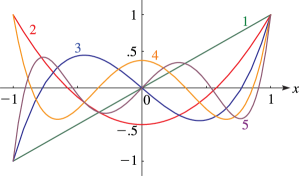
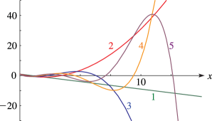
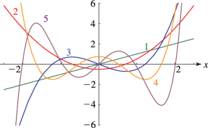
►For $P_n\left(x\right)$ ($={𝖯}_n\left(x\right)$) see §14.33. ►Abramowitz and Stegun (1964, Tables 22.4, 22.6, 22.11, and 22.13) tabulates $T_n\left(x\right)$, $U_n\left(x\right)$, $L_n\left(x\right)$, and $H_n\left(x\right)$ for $n=0(1)12$. The ranges of $x$ are $0.2(.2)1$ for $T_n\left(x\right)$ and $U_n\left(x\right)$, and $0.5,1,3,5,10$ for $L_n\left(x\right)$ and $H_n\left(x\right)$. … ►For $P_n\left(x\right)$, $L_n\left(x\right)$, and $H_n\left(x\right)$ see §3.5(v). …