improved%20accuracy%20via%20numerical%20transformations

(0.004 seconds)

21—30 of 431 matching pages

21: 9.17 Methods of Computation

… в–єSince these expansions diverge, the accuracy they yield is limited by the magnitude of

|z|

. However, in the case of

\operatorname{Ai}\left(z\right)

and

\operatorname{Bi}\left(z\right)

this accuracy can be increased considerably by use of the exponentially-improved forms of expansion supplied in §9.7(v). … в–єA comprehensive and powerful approach is to integrate the defining differential equation (9.2.1) by direct numerical methods. … в–є

§9.17(iv) Via Bessel Functions

… в–єZeros of the Airy functions, and their derivatives, can be computed to high precision via Newton’s rule (§3.8(ii)) or Halley’s rule (§3.8(v)), using values supplied by the asymptotic expansions of §9.9(iv) as initial approximations. …

22: 6.20 Approximations

… в–є

•

Cody and Thacher (1968) provides minimax rational approximations for $E_{1}\left(x\right)$ , with accuracies up to 20S.

в–є

•

Cody and Thacher (1969) provides minimax rational approximations for $\operatorname{Ei}\left(x\right)$ , with accuracies up to 20S.

в–є

•

MacLeod (1996b) provides rational approximations for the sine and cosine integrals and for the auxiliary functions $\mathrm{f}$ and $\mathrm{g}$ , with accuracies up to 20S.

…

23: 27.17 Other Applications

§27.17 Other Applications

в–єReed et al. (1990, pp. 458–470) describes a number-theoretic approach to Fourier analysis (called the arithmetic Fourier transform) that uses the Möbius inversion (27.5.7) to increase efficiency in computing coefficients of Fourier series. … в–єSchroeder (2006) describes many of these applications, including the design of concert hall ceilings to scatter sound into broad lateral patterns for improved acoustic quality, precise measurements of delays of radar echoes from Venus and Mercury to confirm one of the relativistic effects predicted by Einstein’s theory of general relativity, and the use of primes in creating artistic graphical designs.

24: 8 Incomplete Gamma and Related
Functions

…

25: 28 Mathieu Functions and Hill’s Equation

…

26: Errata

… в–єThis update also includes improvments for Chapters 5, 10, 17, 19 and 32. … в–є

Usability

Linkage of mathematical symbols to their definitions were corrected or improved.

… в–є

Equation (14.15.23)

Four of the terms were rewritten for improved clarity.

… в–є

Equations (4.45.8), (4.45.9)

These equations have been rewritten to improve the numerical computation of $\operatorname{arctan}x$ .

… в–є

Chapters 8, 20, 36

Several new equations have been added. See (8.17.24), (20.7.34), §20.11(v), (26.12.27), (36.2.28), and (36.2.29).

…

27: 8.26 Tables

… в–є

•

Khamis (1965) tabulates $P\left(a,x\right)$ for $a=0.05(.05)10(.1)20(.25)70$ , $0.0001\leq x\leq 250$ to 10D.

… в–є

•

Abramowitz and Stegun (1964, pp. 245–248) tabulates $E_{n}\left(x\right)$ for $n=2,3,4,10,20$ , $x=0(.01)2$ to 7D; also $(x+n)e^{x}E_{n}\left(x\right)$ for $n=2,3,4,10,20$ , $x^{-1}=0(.01)0.1(.05)0.5$ to 6S.

… в–є

•

Pagurova (1961) tabulates $E_{n}\left(x\right)$ for $n=0(1)20$ , $x=0(.01)2(.1)10$ to 4-9S; $e^{x}E_{n}\left(x\right)$ for $n=2(1)10$ , $x=10(.1)20$ to 7D; $e^{x}E_{p}\left(x\right)$ for $p=0(.1)1$ , $x=0.01(.01)7(.05)12(.1)20$ to 7S or 7D.

… в–є

•

Zhang and Jin (1996, Table 19.1) tabulates $E_{n}\left(x\right)$ for $n=1,2,3,5,10,15,20$ , $x=0(.1)1,1.5,2,3,5,10,20,30,50,100$ to 7D or 8S.

28: 23 Weierstrass Elliptic and Modular
Functions

…

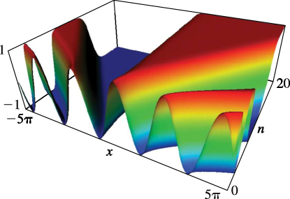
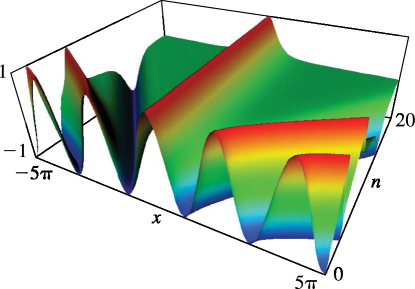
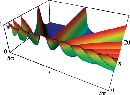
29: 22.3 Graphics

… в–є

See accompanying text — Figure 22.3.13: $\operatorname{sn}\left(x,k\right)$ for $k=1-e^{-n}$ , $n=0$ to 20, $-5\pi\leq x\leq 5\pi$ . Magnify 3D Help

в–є

… в–є

…

30: 5.11 Asymptotic Expansions

… в–єWrench (1968) gives exact values of

g_{k}

up to

g_{20}

. … в–є

§5.11(ii) Error Bounds and Exponential Improvement

… в–єFor error bounds for (5.11.8) and an exponentially-improved extension, see Nemes (2013b). … в–єFor re-expansions of the remainder terms in (5.11.1) and (5.11.3) in series of incomplete gamma functions with exponential improvement (§2.11(iii)) in the asymptotic expansions, see Berry (1991), Boyd (1994), and Paris and Kaminski (2001, §6.4). …

improved%20accuracy%20via%20numerical%20transformations

21—30 of 431 matching pages

21: 9.17 Methods of Computation

§9.17(iv) Via Bessel Functions

22: 6.20 Approximations

23: 27.17 Other Applications

§27.17 Other Applications

24: 8 Incomplete Gamma and Related Functions

25: 28 Mathieu Functions and Hill’s Equation

26: Errata

27: 8.26 Tables

28: 23 Weierstrass Elliptic and Modular Functions

29: 22.3 Graphics

30: 5.11 Asymptotic Expansions

§5.11(ii) Error Bounds and Exponential Improvement

24: 8 Incomplete Gamma and Related
Functions

28: 23 Weierstrass Elliptic and Modular
Functions