had%C3%A9%20approximations

(0.002 seconds)

11—20 of 251 matching pages

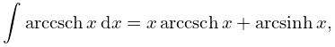
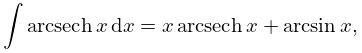
11: 4.40 Integrals

… ►

4.40.14

\int\operatorname{arccsch}x\,\mathrm{d}x=x\operatorname{arccsch}x+% \operatorname{arcsinh}x,

0<x<\infty

ⓘ

Symbols:: $\,\mathrm{d}\NVar{x}$ : differential of $x$ , $\operatorname{arccsch}\NVar{z}$ : inverse hyperbolic cosecant function, $\operatorname{arcsinh}\NVar{z}$ : inverse hyperbolic sine function, $\int$ : integral and $x$ : real variable
A&S Ref:: 4.6.46 (modified. The first printing had an error.)
Permalink:: http://dlmf.nist.gov/4.40.E14
Encodings:: pMML, png, TeX
See also:: Annotations for §4.40(iv), §4.40 and Ch.4

►

4.40.15

\int\operatorname{arcsech}x\,\mathrm{d}x=x\operatorname{arcsech}x+% \operatorname{arcsin}x,

0<x<1

ⓘ

Symbols:: $\,\mathrm{d}\NVar{x}$ : differential of $x$ , $\operatorname{arcsech}\NVar{z}$ : inverse hyperbolic secant function, $\int$ : integral, $\operatorname{arcsin}\NVar{z}$ : arcsine function and $x$ : real variable
A&S Ref:: 4.6.47 (modified. The first printing had an error.)
Permalink:: http://dlmf.nist.gov/4.40.E15
Encodings:: pMML, png, TeX
See also:: Annotations for §4.40(iv), §4.40 and Ch.4

…

… ►The project had two equally important goals: to develop an authoritative replacement for the highly successful Handbook of Mathematical Functions with Formulas, Graphs, and Mathematical Tables, published in 1964 by the National Bureau of Standards (M. …

13: 7.24 Approximations

§7.24 Approximations

►

§7.24(i) Approximations in Terms of Elementary Functions

… ►

•

Cody (1969) provides minimax rational approximations for $\operatorname{erf}x$ and $\operatorname{erfc}x$ . The maximum relative precision is about 20S.

►

•

Cody (1968) gives minimax rational approximations for the Fresnel integrals (maximum relative precision 19S); for a Fortran algorithm and comments see Snyder (1993).

►

•

Cody et al. (1970) gives minimax rational approximations to Dawson’s integral $F\left(x\right)$ (maximum relative precision 20S–22S).

…

14: 25.20 Approximations

§25.20 Approximations

►

•

Cody et al. (1971) gives rational approximations for $\zeta\left(s\right)$ in the form of quotients of polynomials or quotients of Chebyshev series. The ranges covered are $0.5\leq s\leq 5$ , $5\leq s\leq 11$ , $11\leq s\leq 25$ , $25\leq s\leq 55$ . Precision is varied, with a maximum of 20S.

►

•

Piessens and Branders (1972) gives the coefficients of the Chebyshev-series expansions of $s\zeta\left(s+1\right)$ and $\zeta\left(s+k\right)$ , $k=2,3,4,5,8$ , for $0\leq s\leq 1$ (23D).

… ►

•

Morris (1979) gives rational approximations for $\operatorname{Li}_{2}\left(x\right)$ (§25.12(i)) for $0.5\leq x\leq 1$ . Precision is varied with a maximum of 24S.

►

•

Antia (1993) gives minimax rational approximations for $\Gamma\left(s+1\right)F_{s}(x)$ , where $F_{s}(x)$ is the Fermi–Dirac integral (25.12.14), for the intervals $-\infty<x\leq 2$ and $2\leq x<\infty$ , with $s=-\frac{1}{2},\frac{1}{2},\frac{3}{2},\frac{5}{2}$ . For each $s$ there are three sets of approximations, with relative maximum errors $10^{-4},10^{-8},10^{-12}$ .

15: Errata

… ►

Equation (35.7.8)

Originally had the constraint $\Re\left(c\right),\Re\left(c-a-b\right)>\frac{1}{2}(m-1)$ . This constraint was replaced with $\boldsymbol{{0}}<\mathbf{T}<\mathbf{I}$ ; ${\frac{1}{2}}(j+1)-a\in\mathbb{N}$ for some $j=1,\ldots,m$ ; ${\frac{1}{2}}(j+1)-c\notin\mathbb{N}$ and $c-a-b-{\frac{1}{2}}(m-j)\notin\mathbb{N}$ for all $j=1,\ldots,m$ .

►

General

Several biographies had their publications updated.

… ►

Graphics

A software bug that had corrupted some figures, such as those in About Color Map, has been corrected.

… ►

Table 5.4.1

The table of extrema for the Euler gamma function $\Gamma$ had several entries in the $x_{n}$ column that were wrong in the last 2 or 3 digits. These have been corrected and 10 extra decimal places have been included.

$n$	$x_{n}$	$\Gamma\left(x_{n}\right)$
0	$1.46163\;21449\;68362\;34126$	$0.88560\;31944\;10888\;70028$
1	$-0.50408\;30082\;64455\;40926$	$-3.54464\;36111\;55005\;08912$
2	$-1.57349\;84731\;62390\;45878$	$2.30240\;72583\;39680\;13582$
3	$-2.61072\;08684\;44144\;65000$	$-0.88813\;63584\;01241\;92010$
4	$-3.63529\;33664\;36901\;09784$	$0.24512\;75398\;34366\;25044$
5	$-4.65323\;77617\;43142\;44171$	$-0.05277\;96395\;87319\;40076$
6	$-5.66716\;24415\;56885\;53585$	$0.00932\;45944\;82614\;85052$
7	$-6.67841\;82130\;73426\;74283$	$-0.00139\;73966\;08949\;76730$
8	$-7.68778\;83250\;31626\;03744$	$0.00018\;18784\;44909\;40419$
9	$-8.69576\;41638\;16401\;26649$	$-0.00002\;09252\;90446\;52667$
10	$-9.70267\;25400\;01863\;73608$	$0.00000\;21574\;16104\;52285$

Reported 2018-02-17 by David Smith.

… ►

Paragraph Mellin–Barnes Integrals (in §8.6(ii))

The descriptions for the paths of integration of the Mellin-Barnes integrals (8.6.10)–(8.6.12) have been updated. The description for (8.6.11) now states that the path of integration is to the right of all poles. Previously it stated incorrectly that the path of integration had to separate the poles of the gamma function from the pole at $s=0$ . The paths of integration for (8.6.10) and (8.6.12) have been clarified. In the case of (8.6.10), it separates the poles of the gamma function from the pole at $s=a$ for $\gamma\left(a,z\right)$ . In the case of (8.6.12), it separates the poles of the gamma function from the poles at $s=0,1,2,\ldots$ .

Reported 2017-07-10 by Kurt Fischer.

…

16: 6.20 Approximations

§6.20 Approximations

►

§6.20(i) Approximations in Terms of Elementary Functions

… ►

•

Cody and Thacher (1968) provides minimax rational approximations for $E_{1}\left(x\right)$ , with accuracies up to 20S.

►

•

Cody and Thacher (1969) provides minimax rational approximations for $\operatorname{Ei}\left(x\right)$ , with accuracies up to 20S.

►

•

MacLeod (1996b) provides rational approximations for the sine and cosine integrals and for the auxiliary functions $\mathrm{f}$ and $\mathrm{g}$ , with accuracies up to 20S.

…

17: 8.6 Integral Representations

…

18: 25.2 Definition and Expansions

… ►

25.2.4

\zeta\left(s\right)=\frac{1}{s-1}+\sum_{n=0}^{\infty}\frac{(-1)^{n}}{n!}\gamma% _{n}(s-1)^{n},

ⓘ

Symbols:: $\zeta\left(\NVar{s}\right)$ : Riemann zeta function, $\gamma_{\NVar{n}}$ : Stieltjes constants, $!$ : factorial (as in $n!$ ), $\Re$ : real part, $n$ : nonnegative integer and $s$ : complex variable
Keywords:: infinite series, Laurent series
Sources:: Hardy (1912, p. 216); mistakenly missing factor of $(-1)^{n}/n!$ ; Ivić (1985, (1.11), p. 4)
A&S Ref:: 23.2.5 (with unnecessary constraint removed)
Referenced by:: Erratum (V1.0.17) for Equation (25.2.4), Erratum (V1.0.23) for Subsection 25.2(ii) Other Infinite Series
Permalink:: http://dlmf.nist.gov/25.2.E4
Encodings:: pMML, png, TeX
Clarification (effective with 1.0.17):: Originally this equation had the constraint $\Re s>0$ . This constraint is unnecessary because, as stated after (25.2.1), $\zeta\left(s\right)$ is meromorphic with a simple pole at $s=1$ .
Suggested 2017-12-05 by John Harper
See also:: Annotations for §25.2(ii), §25.2 and Ch.25

…

19: 16.26 Approximations

§16.26 Approximations

►For discussions of the approximation of generalized hypergeometric functions and the Meijer

G

-function in terms of polynomials, rational functions, and Chebyshev polynomials see Luke (1975, §§5.12 - 5.13) and Luke (1977b, Chapters 1 and 9).

20: 31.13 Asymptotic Approximations

§31.13 Asymptotic Approximations

►For asymptotic approximations for the accessory parameter eigenvalues

q_{m}

, see Fedoryuk (1991) and Slavyanov (1996). ►For asymptotic approximations of the solutions of Heun’s equation (31.2.1) when two singularities are close together, see Lay and Slavyanov (1999). ►For asymptotic approximations of the solutions of confluent forms of Heun’s equation in the neighborhood of irregular singularities, see Komarov et al. (1976), Ronveaux (1995, Parts B,C,D,E), Bogush and Otchik (1997), Slavyanov and Veshev (1997), and Lay et al. (1998).