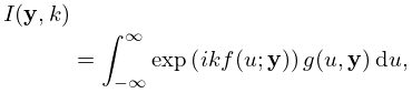
functions f(ϵ,ℓ;r),h(ϵ,ℓ;r)

(0.017 seconds)

31—40 of 443 matching pages

32: Bille C. Carlson

… ►In his paper Lauricella’s hypergeometric function

F_{D}

(1963), he defined the

R

-function, a multivariate hypergeometric function that is homogeneous in its variables, each variable being paired with a parameter. …

33: 33.13 Complex Variable and Parameters

… ►The functions

F_{\ell}\left(\eta,\rho\right)

G_{\ell}\left(\eta,\rho\right)

, and

{H^{\pm}_{\ell}}\left(\eta,\rho\right)

may be extended to noninteger values of

\ell

by generalizing

(2\ell+1)!=\Gamma\left(2\ell+2\right)

, and supplementing (33.6.5) by a formula derived from (33.2.8) with

U\left(a,b,z\right)

expanded via (13.2.42). …

34: 28.30 Expansions in Series of Eigenfunctions

… ►Then every continuous

2\pi

-periodic function

f(x)

whose second derivative is square-integrable over the interval

[0,2\pi]

can be expanded in a uniformly and absolutely convergent series …

35: 33.2 Definitions and Basic Properties

… ►

§33.2(ii) Regular Solution $F_{\ell}\left(\eta,\rho\right)$

►The function

F_{\ell}\left(\eta,\rho\right)

is recessive (§2.7(iii)) at

\rho=0

, and is defined by … ►

F_{\ell}\left(\eta,\rho\right)

is a real and analytic function of

\rho

on the open interval

0<\rho<\infty

, and also an analytic function of

\eta

when

-\infty<\eta<\infty

. … ►

§33.2(iii) Irregular Solutions $G_{\ell}\left(\eta,\rho\right),{H^{\pm}_{\ell}}\left(\eta,\rho\right)$

… ►As in the case of

F_{\ell}\left(\eta,\rho\right)

, the solutions

{H^{\pm}_{\ell}}\left(\eta,\rho\right)

and

G_{\ell}\left(\eta,\rho\right)

are analytic functions of

\rho

when

0<\rho<\infty

. …

36: 36.12 Uniform Approximation of Integrals

… ►

36.12.1

I(\mathbf{y},k)=\int_{-\infty}^{\infty}\exp\left(ikf(u;\mathbf{y})\right)g(u,% \mathbf{y})\,\mathrm{d}u,

ⓘ

Defines:: $I(\mathbf{y},k)$ : oscillatory integral (locally)
Symbols:: $\,\mathrm{d}\NVar{x}$ : differential of $x$ , $\exp\NVar{z}$ : exponential function, $\mathrm{i}$ : imaginary unit, $\int$ : integral, $k$ : variable, $g(u,\mathbf{y})$ : function, $f(u,\mathbf{y})$ : function and $u(t;\mathbf{y})$ : mapping
Referenced by:: §36.13
Permalink:: http://dlmf.nist.gov/36.12.E1
Encodings:: pMML, png, TeX
See also:: Annotations for §36.12(i), §36.12 and Ch.36

… ►As

\mathbf{y}

varies as many as

K+1

(real or complex) critical points of the smooth phase function

f

can coalesce in clusters of two or more. …Also,

f

is real analytic, and

\ifrac{{\partial}^{K+2}f}{{\partial u}^{K+2}}>0

for all

\mathbf{y}

such that all

K+1

critical points coincide. … ►with the

K+1

functions

A(\mathbf{y})

and

\mathbf{x}(\mathbf{y})

determined by correspondence of the

K+1

critical points of

f

and

\Phi_{K}

. … ►

36.12.6

A(\mathbf{y})=f(u(0,\mathbf{y});\mathbf{y}),

ⓘ

Defines:: $A(\mathbf{y})$ : function (locally)
Symbols:: $f(u,\mathbf{y})$ : function and $u(t;\mathbf{y})$ : mapping
Permalink:: http://dlmf.nist.gov/36.12.E6
Encodings:: pMML, png, TeX
See also:: Annotations for §36.12(i), §36.12 and Ch.36

…

Hastings (1955) gives several minimax polynomial and rational approximations for $E_{1}\left(x\right)+\ln x$ , $xe^{x}E_{1}\left(x\right)$ , and the auxiliary functions $\mathrm{f}\left(x\right)$ and $\mathrm{g}\left(x\right)$ . These are included in Abramowitz and Stegun (1964, Ch. 5).

… ►

•

MacLeod (1996b) provides rational approximations for the sine and cosine integrals and for the auxiliary functions $\mathrm{f}$ and $\mathrm{g}$ , with accuracies up to 20S.

… ►

•

Luke (1969b, p. 25) gives a Chebyshev expansion near infinity for the confluent hypergeometric $U$ -function (§13.2(i)) from which Chebyshev expansions near infinity for $E_{1}\left(z\right)$ , $\mathrm{f}\left(z\right)$ , and $\mathrm{g}\left(z\right)$ follow by using (6.11.2) and (6.11.3). Luke also includes a recursion scheme for computing the coefficients in the expansions of the $U$ functions. If $|\operatorname{ph}z|<\pi$ the scheme can be used in backward direction.

…

38: 16.12 Products

… ►

16.12.1

{{}_{0}F_{1}}\left(-;a;z\right){{}_{0}F_{1}}\left(-;b;z\right)={{}_{2}F_{3}}% \left({\frac{1}{2}(a+b),\frac{1}{2}(a+b-1)\atop a,b,a+b-1};4z\right).

ⓘ

Symbols:: ${{}_{\NVar{p}}F_{\NVar{q}}}\left(\NVar{a_{1},\dots,a_{p}};\NVar{b_{1},\dots,b_% {q}};\NVar{z}\right)$ or ${{}_{\NVar{p}}F_{\NVar{q}}}\left({\NVar{a_{1},\dots,a_{p}}\atop\NVar{b_{1},% \dots,b_{q}}};\NVar{z}\right)$ : alternatively ${{}_{\NVar{p}}F_{\NVar{q}}}\left(\NVar{\mathbf{a}};\NVar{\mathbf{b}};\NVar{z}\right)$ or ${{}_{\NVar{p}}F_{\NVar{q}}}\left({\NVar{\mathbf{a}}\atop\NVar{\mathbf{b}}};% \NVar{z}\right)$
generalized hypergeometric function, $z$ : complex variable, $a,a_{1},\ldots,a_{p}$ : real or complex parameters and $b,b_{1},\ldots,b_{q}$ : real or complex parameters
Referenced by:: (10.8.3), §10.8, §10.8, §16.12, Erratum (V1.0.17) for Section 10.8
Permalink:: http://dlmf.nist.gov/16.12.E1
Encodings:: pMML, png, TeX
See also:: Annotations for §16.12 and Ch.16

… ►

16.12.2

\left({{}_{2}F_{1}}\left({a,b\atop a+b+\frac{1}{2}};z\right)\right)^{2}={{}_{3% }F_{2}}\left({2a,2b,a+b\atop a+b+\frac{1}{2},2a+2b};z\right).

ⓘ

Symbols:: ${{}_{2}F_{1}}\left(\NVar{a},\NVar{b};\NVar{c};\NVar{z}\right)$ : $=F\left(\NVar{a},\NVar{b};\NVar{c};\NVar{z}\right)$ notation for Gauss’ hypergeometric function, ${{}_{\NVar{p}}F_{\NVar{q}}}\left(\NVar{a_{1},\dots,a_{p}};\NVar{b_{1},\dots,b_% {q}};\NVar{z}\right)$ or ${{}_{\NVar{p}}F_{\NVar{q}}}\left({\NVar{a_{1},\dots,a_{p}}\atop\NVar{b_{1},% \dots,b_{q}}};\NVar{z}\right)$ : alternatively ${{}_{\NVar{p}}F_{\NVar{q}}}\left(\NVar{\mathbf{a}};\NVar{\mathbf{b}};\NVar{z}\right)$ or ${{}_{\NVar{p}}F_{\NVar{q}}}\left({\NVar{\mathbf{a}}\atop\NVar{\mathbf{b}}};% \NVar{z}\right)$
generalized hypergeometric function, $z$ : complex variable, $a,a_{1},\ldots,a_{p}$ : real or complex parameters and $b,b_{1},\ldots,b_{q}$ : real or complex parameters
Referenced by:: §16.12, §17.9(iii), Erratum (V1.1.12) for Subsection 17.9(iii)
Permalink:: http://dlmf.nist.gov/16.12.E2
Encodings:: pMML, png, TeX
See also:: Annotations for §16.12 and Ch.16

… ►

16.12.3

\left({{}_{2}F_{1}}\left({a,b\atop c};z\right)\right)^{2}=\sum_{k=0}^{\infty}% \frac{{\left(2a\right)_{k}}{\left(2b\right)_{k}}{\left(c-\frac{1}{2}\right)_{k% }}}{{\left(c\right)_{k}}{\left(2c-1\right)_{k}}k!}{{}_{4}F_{3}}\left({-\frac{1% }{2}k,\frac{1}{2}(1-k),a+b-c+\frac{1}{2},\frac{1}{2}\atop a+\frac{1}{2},b+% \frac{1}{2},\frac{3}{2}-k-c};1\right)z^{k},

|z|<1

ⓘ

Symbols:: ${{}_{2}F_{1}}\left(\NVar{a},\NVar{b};\NVar{c};\NVar{z}\right)$ : $=F\left(\NVar{a},\NVar{b};\NVar{c};\NVar{z}\right)$ notation for Gauss’ hypergeometric function, ${{}_{\NVar{p}}F_{\NVar{q}}}\left(\NVar{a_{1},\dots,a_{p}};\NVar{b_{1},\dots,b_% {q}};\NVar{z}\right)$ or ${{}_{\NVar{p}}F_{\NVar{q}}}\left({\NVar{a_{1},\dots,a_{p}}\atop\NVar{b_{1},% \dots,b_{q}}};\NVar{z}\right)$ : alternatively ${{}_{\NVar{p}}F_{\NVar{q}}}\left(\NVar{\mathbf{a}};\NVar{\mathbf{b}};\NVar{z}\right)$ or ${{}_{\NVar{p}}F_{\NVar{q}}}\left({\NVar{\mathbf{a}}\atop\NVar{\mathbf{b}}};% \NVar{z}\right)$
generalized hypergeometric function, ${\left(\NVar{a}\right)_{\NVar{n}}}$ : Pochhammer’s symbol (or shifted factorial), $!$ : factorial (as in $n!$ ), $z$ : complex variable, $a,a_{1},\ldots,a_{p}$ : real or complex parameters and $b,b_{1},\ldots,b_{q}$ : real or complex parameters
Referenced by:: §16.12
Permalink:: http://dlmf.nist.gov/16.12.E3
Encodings:: pMML, png, TeX
See also:: Annotations for §16.12 and Ch.16

…

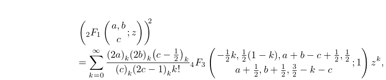
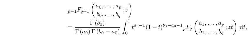
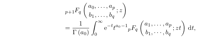
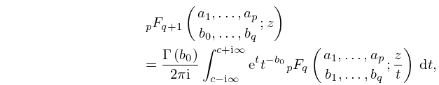
39: 16.5 Integral Representations and Integrals

… ►

16.5.1

\left({\textstyle\ifrac{\prod\limits_{k=1}^{p}\Gamma\left(a_{k}\right)}{\prod% \limits_{k=1}^{q}\Gamma\left(b_{k}\right)}}\right){{}_{p}F_{q}}\left({a_{1},% \dots,a_{p}\atop b_{1},\dots,b_{q}};z\right)=\frac{1}{2\pi\mathrm{i}}\int_{L}% \left({\textstyle\ifrac{\prod\limits_{k=1}^{p}\Gamma\left(a_{k}+s\right)}{% \prod\limits_{k=1}^{q}\Gamma\left(b_{k}+s\right)}}\right)\Gamma\left(-s\right)% (-z)^{s}\,\mathrm{d}s,

ⓘ

Symbols:: $\Gamma\left(\NVar{z}\right)$ : gamma function, ${{}_{\NVar{p}}F_{\NVar{q}}}\left(\NVar{a_{1},\dots,a_{p}};\NVar{b_{1},\dots,b_% {q}};\NVar{z}\right)$ or ${{}_{\NVar{p}}F_{\NVar{q}}}\left({\NVar{a_{1},\dots,a_{p}}\atop\NVar{b_{1},% \dots,b_{q}}};\NVar{z}\right)$ : alternatively ${{}_{\NVar{p}}F_{\NVar{q}}}\left(\NVar{\mathbf{a}};\NVar{\mathbf{b}};\NVar{z}\right)$ or ${{}_{\NVar{p}}F_{\NVar{q}}}\left({\NVar{\mathbf{a}}\atop\NVar{\mathbf{b}}};% \NVar{z}\right)$
generalized hypergeometric function, $\pi$ : the ratio of the circumference of a circle to its diameter, $\,\mathrm{d}\NVar{x}$ : differential of $x$ , $\mathrm{i}$ : imaginary unit, $\int$ : integral, $p$ : nonnegative integer, $q$ : nonnegative integer, $z$ : complex variable, $a,a_{1},\ldots,a_{p}$ : real or complex parameters and $b,b_{1},\ldots,b_{q}$ : real or complex parameters
Referenced by:: §13.6(vi), §16.11(i), §16.5, §16.5
Permalink:: http://dlmf.nist.gov/16.5.E1
Encodings:: pMML, png, TeX
See also:: Annotations for §16.5 and Ch.16

… ►In this event, the formal power-series expansion of the left-hand side (obtained from (16.2.1)) is the asymptotic expansion of the right-hand side as

z\to 0

in the sector

|\operatorname{ph}\left(-z\right)|\leq(p+1-q-\delta)\pi/2

, where

\delta

is an arbitrary small positive constant. … ►

16.5.2

{{}_{p+1}F_{q+1}}\left({a_{0},\dots,a_{p}\atop b_{0},\dots,b_{q}};z\right)=% \frac{\Gamma\left(b_{0}\right)}{\Gamma\left(a_{0}\right)\Gamma\left(b_{0}-a_{0% }\right)}\int_{0}^{1}t^{a_{0}-1}(1-t)^{b_{0}-a_{0}-1}{{}_{p}F_{q}}\left({a_{1}% ,\dots,a_{p}\atop b_{1},\dots,b_{q}};zt\right)\,\mathrm{d}t,

\Re b_{0}>\Re a_{0}>0

ⓘ

Symbols:: $\Gamma\left(\NVar{z}\right)$ : gamma function, ${{}_{\NVar{p}}F_{\NVar{q}}}\left(\NVar{a_{1},\dots,a_{p}};\NVar{b_{1},\dots,b_% {q}};\NVar{z}\right)$ or ${{}_{\NVar{p}}F_{\NVar{q}}}\left({\NVar{a_{1},\dots,a_{p}}\atop\NVar{b_{1},% \dots,b_{q}}};\NVar{z}\right)$ : alternatively ${{}_{\NVar{p}}F_{\NVar{q}}}\left(\NVar{\mathbf{a}};\NVar{\mathbf{b}};\NVar{z}\right)$ or ${{}_{\NVar{p}}F_{\NVar{q}}}\left({\NVar{\mathbf{a}}\atop\NVar{\mathbf{b}}};% \NVar{z}\right)$
generalized hypergeometric function, $\,\mathrm{d}\NVar{x}$ : differential of $x$ , $\int$ : integral, $\Re$ : real part, $p$ : nonnegative integer, $q$ : nonnegative integer, $z$ : complex variable, $a,a_{1},\ldots,a_{p}$ : real or complex parameters and $b,b_{1},\ldots,b_{q}$ : real or complex parameters
Keywords:: Mellin transform
Referenced by:: §16.5, §16.5
Permalink:: http://dlmf.nist.gov/16.5.E2
Encodings:: pMML, png, TeX
See also:: Annotations for §16.5 and Ch.16

►

16.5.3

{{}_{p+1}F_{q}}\left({a_{0},\dots,a_{p}\atop b_{1},\dots,b_{q}};z\right)=\frac% {1}{\Gamma\left(a_{0}\right)}\int_{0}^{\infty}{\mathrm{e}}^{-t}t^{a_{0}-1}{{}_% {p}F_{q}}\left({a_{1},\dots,a_{p}\atop b_{1},\cdots,b_{q}};zt\right)\,\mathrm{% d}t,

\Re z<1

\Re a_{0}>0

ⓘ

Symbols:: $\Gamma\left(\NVar{z}\right)$ : gamma function, ${{}_{\NVar{p}}F_{\NVar{q}}}\left(\NVar{a_{1},\dots,a_{p}};\NVar{b_{1},\dots,b_% {q}};\NVar{z}\right)$ or ${{}_{\NVar{p}}F_{\NVar{q}}}\left({\NVar{a_{1},\dots,a_{p}}\atop\NVar{b_{1},% \dots,b_{q}}};\NVar{z}\right)$ : alternatively ${{}_{\NVar{p}}F_{\NVar{q}}}\left(\NVar{\mathbf{a}};\NVar{\mathbf{b}};\NVar{z}\right)$ or ${{}_{\NVar{p}}F_{\NVar{q}}}\left({\NVar{\mathbf{a}}\atop\NVar{\mathbf{b}}};% \NVar{z}\right)$
generalized hypergeometric function, $\,\mathrm{d}\NVar{x}$ : differential of $x$ , $\mathrm{e}$ : base of natural logarithm, $\int$ : integral, $\Re$ : real part, $p$ : nonnegative integer, $q$ : nonnegative integer, $z$ : complex variable, $a,a_{1},\ldots,a_{p}$ : real or complex parameters and $b,b_{1},\ldots,b_{q}$ : real or complex parameters
Keywords:: Laplace transform, Mellin transform
Referenced by:: §16.5
Permalink:: http://dlmf.nist.gov/16.5.E3
Encodings:: pMML, png, TeX
See also:: Annotations for §16.5 and Ch.16

►

16.5.4

{{}_{p}F_{q+1}}\left({a_{1},\dots,a_{p}\atop b_{0},\dots,b_{q}};z\right)=\frac% {\Gamma\left(b_{0}\right)}{2\pi\mathrm{i}}\int_{c-\mathrm{i}\infty}^{c+\mathrm% {i}\infty}{\mathrm{e}}^{t}t^{-b_{0}}{{}_{p}F_{q}}\left({a_{1},\dots,a_{p}\atop b% _{1},\dots,b_{q}};\frac{z}{t}\right)\,\mathrm{d}t,

c>0

\Re b_{0}>0

ⓘ

Symbols:: $\Gamma\left(\NVar{z}\right)$ : gamma function, ${{}_{\NVar{p}}F_{\NVar{q}}}\left(\NVar{a_{1},\dots,a_{p}};\NVar{b_{1},\dots,b_% {q}};\NVar{z}\right)$ or ${{}_{\NVar{p}}F_{\NVar{q}}}\left({\NVar{a_{1},\dots,a_{p}}\atop\NVar{b_{1},% \dots,b_{q}}};\NVar{z}\right)$ : alternatively ${{}_{\NVar{p}}F_{\NVar{q}}}\left(\NVar{\mathbf{a}};\NVar{\mathbf{b}};\NVar{z}\right)$ or ${{}_{\NVar{p}}F_{\NVar{q}}}\left({\NVar{\mathbf{a}}\atop\NVar{\mathbf{b}}};% \NVar{z}\right)$
generalized hypergeometric function, $\pi$ : the ratio of the circumference of a circle to its diameter, $\,\mathrm{d}\NVar{x}$ : differential of $x$ , $\mathrm{e}$ : base of natural logarithm, $\mathrm{i}$ : imaginary unit, $\int$ : integral, $\Re$ : real part, $p$ : nonnegative integer, $q$ : nonnegative integer, $z$ : complex variable, $a,a_{1},\ldots,a_{p}$ : real or complex parameters and $b,b_{1},\ldots,b_{q}$ : real or complex parameters
Keywords:: Mellin transform
Referenced by:: §16.5, §16.5
Permalink:: http://dlmf.nist.gov/16.5.E4
Encodings:: pMML, png, TeX
See also:: Annotations for §16.5 and Ch.16

…

40: 10.70 Zeros

… ►

10.70.1

\frac{\mu-1}{16t}+\frac{\mu-1}{32t^{2}}+\frac{(\mu-1)(5\mu+19)}{1536t^{3}}+% \frac{3(\mu-1)^{2}}{512t^{4}}+\dotsi.

ⓘ

Defines:: $f(t)$ : function (locally)
A&S Ref:: 9.10.35
Referenced by:: §10.70
Permalink:: http://dlmf.nist.gov/10.70.E1
Encodings:: pMML, png, TeX
See also:: Annotations for §10.70 and Ch.10

…

functions f(ϵ,ℓ;r),h(ϵ,ℓ;r)

31—40 of 443 matching pages

31: 33.15 Graphics

§33.15(i) Line Graphs of the Coulomb Functions $f\left(\epsilon,\ell;r\right)$ and $h\left(\epsilon,\ell;r\right)$

§33.15(ii) Surfaces of the Coulomb Functions $f\left(\epsilon,\ell;r\right)$ , $h\left(\epsilon,\ell;r\right)$ , $s\left(\epsilon,\ell;r\right)$ , and $c\left(\epsilon,\ell;r\right)$

32: Bille C. Carlson

33: 33.13 Complex Variable and Parameters

34: 28.30 Expansions in Series of Eigenfunctions

35: 33.2 Definitions and Basic Properties

§33.2(ii) Regular Solution $F_{\ell}\left(\eta,\rho\right)$

§33.2(iii) Irregular Solutions $G_{\ell}\left(\eta,\rho\right),{H^{\pm}_{\ell}}\left(\eta,\rho\right)$

36: 36.12 Uniform Approximation of Integrals

37: 6.20 Approximations

38: 16.12 Products

39: 16.5 Integral Representations and Integrals

40: 10.70 Zeros

functions f(ϵ,ℓ;r),h(ϵ,ℓ;r)

31—40 of 443 matching pages

31: 33.15 Graphics

§33.15(i) Line Graphs of the Coulomb Functions f ⁡ ( ϵ , ℓ ; r ) and h ⁡ ( ϵ , ℓ ; r )

§33.15(ii) Surfaces of the Coulomb Functions f ⁡ ( ϵ , ℓ ; r ) , h ⁡ ( ϵ , ℓ ; r ) , s ⁡ ( ϵ , ℓ ; r ) , and c ⁡ ( ϵ , ℓ ; r )

32: Bille C. Carlson

33: 33.13 Complex Variable and Parameters

34: 28.30 Expansions in Series of Eigenfunctions

35: 33.2 Definitions and Basic Properties

§33.2(ii) Regular Solution F ℓ ⁡ ( η , ρ )

§33.2(iii) Irregular Solutions G ℓ ⁡ ( η , ρ ) , H ℓ ± ⁡ ( η , ρ )

36: 36.12 Uniform Approximation of Integrals

37: 6.20 Approximations

38: 16.12 Products

39: 16.5 Integral Representations and Integrals

40: 10.70 Zeros

§33.15(i) Line Graphs of the Coulomb Functions $f\left(\epsilon,\ell;r\right)$ and $h\left(\epsilon,\ell;r\right)$

§33.15(ii) Surfaces of the Coulomb Functions $f\left(\epsilon,\ell;r\right)$ , $h\left(\epsilon,\ell;r\right)$ , $s\left(\epsilon,\ell;r\right)$ , and $c\left(\epsilon,\ell;r\right)$

§33.2(ii) Regular Solution $F_{\ell}\left(\eta,\rho\right)$

§33.2(iii) Irregular Solutions $G_{\ell}\left(\eta,\rho\right),{H^{\pm}_{\ell}}\left(\eta,\rho\right)$