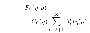
functions Fℓ(η,ρ),Gℓ(η,ρ),H±ℓ(η,ρ)
(0.013 seconds)
11—20 of 236 matching pages
11: Bille C. Carlson
…
►In his paper Lauricella’s hypergeometric function
(1963), he defined the -function, a multivariate hypergeometric function that is homogeneous in its variables, each variable being paired with a parameter.
…
12: 33.13 Complex Variable and Parameters
…
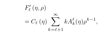
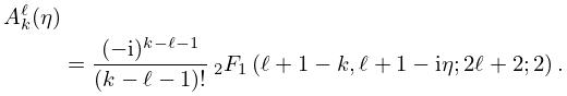
►The functions
, , and may be extended to noninteger values of by generalizing , and supplementing (33.6.5) by a formula derived from (33.2.8) with expanded via (13.2.42).
…
13: 33.2 Definitions and Basic Properties
…
►
§33.2(ii) Regular Solution
►The function is recessive (§2.7(iii)) at , and is defined by … ► is a real and analytic function of on the open interval , and also an analytic function of when . … ►§33.2(iii) Irregular Solutions
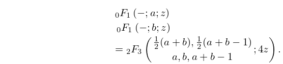
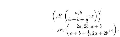
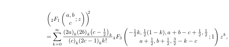
… ►As in the case of , the solutions and are analytic functions of when . …14: 16.12 Products
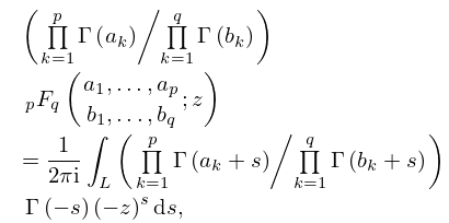
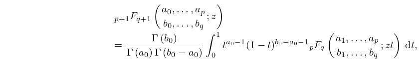
15: 16.5 Integral Representations and Integrals
…
►
16.5.1
…
►In this event, the formal power-series expansion of the left-hand side (obtained from (16.2.1)) is the asymptotic expansion of the right-hand side as in the sector , where is an arbitrary small positive constant.
…
►
16.5.2
,
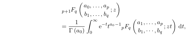
►
16.5.3
, ,
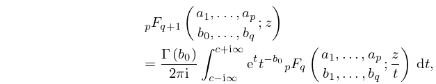
►
16.5.4
, .
…
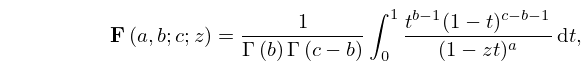
16: 15.6 Integral Representations
…
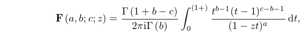
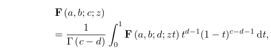
►The function
(not ) has the following integral representations:
►
15.6.1
; .
►
15.6.2
; , .
…
►
15.6.6
; .
…
►
15.6.8
; .
…
17: 16.18 Special Cases
…
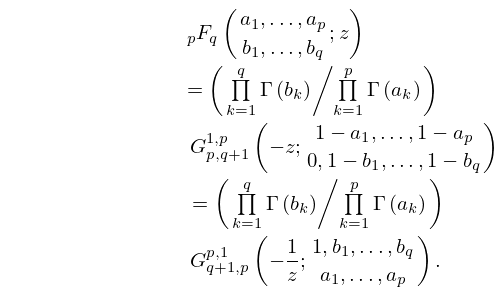
►The and
functions introduced in Chapters 13 and 15, as well as the more general
functions introduced in the present chapter, are all special cases of the Meijer -function.
…
►
16.18.1
►As a corollary, special cases of the and
functions, including Airy functions, Bessel functions, parabolic cylinder functions, Ferrers functions, associated Legendre functions, and many orthogonal polynomials, are all special cases of the Meijer -function.
…
18: 15.4 Special Cases
19: 33.6 Power-Series Expansions in
20: 15.2 Definitions and Analytical Properties
…
►The hypergeometric function
is defined by the Gauss series
…
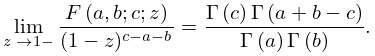
►The principal branch of is an entire function of , , and .
…As a multivalued function of , is analytic everywhere except for possible branch points at , , and .
The same properties hold for , except that as a function of , in general has poles at .
…
►For example, when , , and , is a polynomial:
…
