for derivatives

SearchAdvancedHelp

(0.003 seconds)

21—30 of 277 matching pages

21: 10.51 Recurrence Relations and Derivatives

§10.51 Recurrence Relations and Derivatives

… ►

$${\left(\frac{1}{z}\frac{d}{dz}\right)}^m(z^{n+1}{f}_n(z))=z^{n-m+1}{f}_{n-m}(z),$$ $m=0,1,\mathrm{\dots },n$,

►

$${\left(\frac{1}{z}\frac{d}{dz}\right)}^m(z^{-n}{f}_n(z))={(-1)}^m{z}^{-n-m}{f}_{n+m}(z),$$ $m=0,1,\mathrm{\dots }.$

… ►

$${\left(\frac{1}{z}\frac{d}{dz}\right)}^m(z^{n+1}{g}_n(z))=z^{n-m+1}{g}_{n-m}(z),$$ $m=0,1,\mathrm{\dots },n$,

►

$${\left(\frac{1}{z}\frac{d}{dz}\right)}^m(z^{-n}{g}_n(z))=z^{-n-m}{g}_{n+m}(z),$$ $m=0,1,\mathrm{\dots }.$

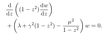
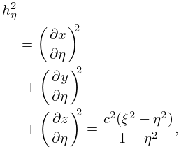
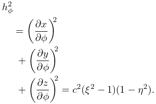
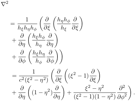
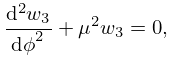
22: 29.11 Lamé Wave Equation

… ►

29.11.1 $$\frac{d^{2}w}{{dz}^2}+(h-\nu (\nu +1)k^2{\mathrm{sn}}^2(z,k)+k^2{\omega }^2{\mathrm{sn}}^4(z,k))w=0,$$

ⓘ

Symbols:

$\mathrm{sn}(z,k)$: Jacobian elliptic function, $\frac{df}{dx}$: derivative of $f$ with respect to $x$ , $z$: complex variable, $h$: real parameter, $k$: real parameter, $\nu$: real parameter, $\omega$: parameter and $w(z)$: solution

Referenced by:

§29.11, §29.11, §29.18(ii), §29.7(ii)

Permalink:

http://dlmf.nist.gov/29.11.E1

Encodings:

pMML, png, TeX

See also:

Annotations for §29.11 and Ch.29

…

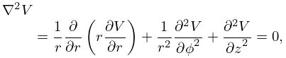
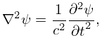
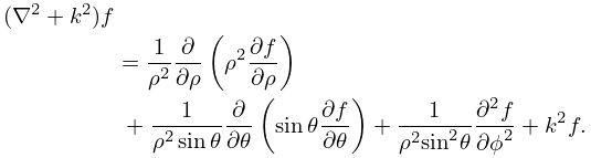
23: 16.14 Partial Differential Equations

… ►

$$x(1-x)\frac{{\partial }^2{F}_1}{{\partial x}^2}+y(1-x)\frac{{\partial }^2{F}_1}{\partial x\partial y}+\left(\gamma -(\alpha +\beta +1)x\right)\frac{\partial F_1}{\partial x}-\beta y\frac{\partial F_1}{\partial y}-\alpha \beta F_1=0,$$

►

$$y(1-y)\frac{{\partial }^2{F}_1}{{\partial y}^2}+x(1-y)\frac{{\partial }^2{F}_1}{\partial x\partial y}+\left(\gamma -(\alpha +{\beta }^{\prime }+1)y\right)\frac{\partial F_1}{\partial y}-{\beta }^{\prime }x\frac{\partial F_1}{\partial x}-\alpha {\beta }^{\prime }{F}_1=0,$$

►

$$x(1-x)\frac{{\partial }^2{F}_2}{{\partial x}^2}-xy\frac{{\partial }^2{F}_2}{\partial x\partial y}+\left(\gamma -(\alpha +\beta +1)x\right)\frac{\partial F_2}{\partial x}-\beta y\frac{\partial F_2}{\partial y}-\alpha \beta F_2=0,$$

… ►

$$x(1-x)\frac{{\partial }^2{F}_4}{{\partial x}^2}-2xy\frac{{\partial }^2{F}_4}{\partial x\partial y}-y^2\frac{{\partial }^2{F}_4}{{\partial y}^2}+\left(\gamma -(\alpha +\beta +1)x\right)\frac{\partial F_4}{\partial x}-(\alpha +\beta +1)y\frac{\partial F_4}{\partial y}-\alpha \beta F_4=0,$$

►

$$y(1-y)\frac{{\partial }^2{F}_4}{{\partial y}^2}-2xy\frac{{\partial }^2{F}_4}{\partial x\partial y}-x^2\frac{{\partial }^2{F}_4}{{\partial x}^2}+\left({\gamma }^{\prime }-(\alpha +\beta +1)y\right)\frac{\partial F_4}{\partial y}-(\alpha +\beta +1)x\frac{\partial F_4}{\partial x}-\alpha \beta F_4=0.$$

…

24: 9.9 Zeros

… ►They are denoted by $a_k$, $a_k^{\prime }$, $b_k$, $b_k^{\prime }$, respectively, arranged in ascending order of absolute value for $k=1,2,\mathrm{\dots }.$ … ►They lie in the sectors and , and are denoted by ${\beta }_k$, ${\beta }_k^{\prime }$, respectively, in the former sector, and by $\overline{{\beta }_k}$, $\overline{{\beta }_k^{\prime }}$, in the conjugate sector, again arranged in ascending order of absolute value (modulus) for $k=1,2,\mathrm{\dots }.$ See §9.3(ii) for visualizations. … ►

§9.9(iii) Derivatives With Respect to $k$

… ►

$\mathrm{Ai}\left(a_k^{\prime }\right)={(-1)}^{k-1}{\left(a_k^{\prime }{\displaystyle \frac{d{a}_k^{\prime }}{dk}}\right)}^{-1/2}.$

… ►For error bounds for the asymptotic expansions of $a_k$, $b_k$, $a_k^{\prime }$, and $b_k^{\prime }$ see Pittaluga and Sacripante (1991), and a conjecture given in Fabijonas and Olver (1999). …

25: 30.2 Differential Equations

… ►

30.2.1 $$\frac{d}{dz}\left((1-z^2)\frac{dw}{dz}\right)+\left(\lambda +{\gamma }^2(1-z^2)-\frac{{\mu }^2}{1-z^2}\right)w=0.$$

ⓘ

Symbols:

$\frac{df}{dx}$: derivative of $f$ with respect to $x$ , $z$: complex variable, $w$: solution to DE, $\lambda$: real parameter, ${\gamma }^2$: real parameter and $\mu$: real parameter

Referenced by:

§30.11(i), §30.12, §30.12, §30.13(iv), §30.14(iv), §30.16(ii), §30.2(ii), §30.2(iii), §30.3(i), §30.4(i), §30.5, §30.6, §30.6

Permalink:

http://dlmf.nist.gov/30.2.E1

Encodings:

pMML, png, TeX

See also:

Annotations for §30.2(i), §30.2 and Ch.30

… ►

30.2.2 $$\frac{d^{2}g}{{dt}^2}+\left(\lambda +\frac{1}{4}+{\gamma }^2{\sin }^{2}t-\frac{{\mu }^2-\frac{1}{4}}{{\sin }^{2}t}\right)g=0,$$

ⓘ

Symbols:

$\frac{df}{dx}$: derivative of $f$ with respect to $x$ , $\sin z$: sine function, $\lambda$: real parameter, ${\gamma }^2$: real parameter and $\mu$: real parameter

Referenced by:

§30.2(iii)

Permalink:

http://dlmf.nist.gov/30.2.E2

Encodings:

pMML, png, TeX

See also:

Annotations for §30.2(ii), §30.2 and Ch.30

… ►

30.2.4 $$({\zeta }^2-{\gamma }^2)\frac{d^{2}w}{{d\zeta }^2}+2\zeta \frac{dw}{d\zeta }+\left({\zeta }^2-\lambda -{\gamma }^2-\frac{{\gamma }^2{\mu }^2}{{\zeta }^2-{\gamma }^2}\right)w=0.$$

ⓘ

Symbols:

$\frac{df}{dx}$: derivative of $f$ with respect to $x$ , $w$: solution to DE, $\lambda$: real parameter, ${\gamma }^2$: real parameter, $\mu$: real parameter and $\zeta$: parameter

Referenced by:

§30.2(iii)

Permalink:

http://dlmf.nist.gov/30.2.E4

Encodings:

pMML, png, TeX

See also:

Annotations for §30.2(ii), §30.2 and Ch.30

…

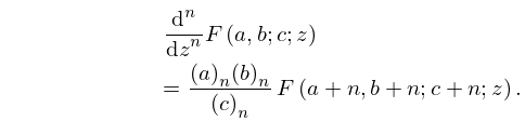
26: 15.5 Derivatives and Contiguous Functions

§15.5 Derivatives and Contiguous Functions

►

§15.5(i) Differentiation Formulas

… ►

15.5.2 $$\frac{d^n}{{dz}^n}F(a,b;c;z)=\frac{{\left(a\right)}_n{\left(b\right)}_n}{{\left(c\right)}_n}F(a+n,b+n;c+n;z).$$

ⓘ

Symbols:

$F(a,b;c;z)$ or $F(\genfrac{}{}{0pt}{}{a,b}{c};z)$: $={}_2{}^{}F_1^{}(a,b;c;z)$ Gauss’ hypergeometric function, ${\left(a\right)}_n$: Pochhammer’s symbol (or shifted factorial), $\frac{df}{dx}$: derivative of $f$ with respect to $x$ , $n$: integer, $z$: complex variable, $a$: real or complex parameter, $b$: real or complex parameter and $c$: real or complex parameter

Permalink:

http://dlmf.nist.gov/15.5.E2

Encodings:

pMML, png, TeX

See also:

Annotations for §15.5(i), §15.5 and Ch.15

… ►

15.5.10 $${\left(z\frac{d}{dz}z\right)}^n=z^n\frac{d^n}{{dz}^n}{z}^n,$$ $n=1,2,3,\mathrm{\dots }$.

ⓘ

Symbols:

$\frac{df}{dx}$: derivative of $f$ with respect to $x$ , $n$: integer and $z$: complex variable

Referenced by:

§15.5(i)

Permalink:

http://dlmf.nist.gov/15.5.E10

Encodings:

pMML, png, TeX

See also:

Annotations for §15.5(i), §15.5 and Ch.15

… ► …

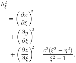
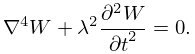
27: 30.13 Wave Equation in Prolate Spheroidal Coordinates

… ►

30.13.3 $$h_{\xi }^2={\left(\frac{\partial x}{\partial \xi }\right)}^2+{\left(\frac{\partial y}{\partial \xi }\right)}^2+{\left(\frac{\partial z}{\partial \xi }\right)}^2=\frac{c^2({\xi }^2-{\eta }^2)}{{\xi }^2-1},$$

ⓘ

Symbols:

$\frac{\partial f}{\partial x}$: partial derivative of $f$ with respect to $x$ , $\partial x$: partial differential of $x$ , $z$: complex variable, $x$: real variable, $y$: real variable, $\xi$: prolate spheroidal coordinate, $\eta$: prolate spheroidal coordinate, $c$: positive constant and $h_{\xi },h_{\eta },h_{\varphi }$: metric coefficients

A&S Ref:

21.4.2

Permalink:

http://dlmf.nist.gov/30.13.E3

Encodings:

pMML, png, TeX

See also:

Annotations for §30.13(ii), §30.13 and Ch.30

►

30.13.4 $$h_{\eta }^2={\left(\frac{\partial x}{\partial \eta }\right)}^2+{\left(\frac{\partial y}{\partial \eta }\right)}^2+{\left(\frac{\partial z}{\partial \eta }\right)}^2=\frac{c^2({\xi }^2-{\eta }^2)}{1-{\eta }^2},$$

ⓘ

Symbols:

$\frac{\partial f}{\partial x}$: partial derivative of $f$ with respect to $x$ , $\partial x$: partial differential of $x$ , $z$: complex variable, $x$: real variable, $y$: real variable, $\xi$: prolate spheroidal coordinate, $\eta$: prolate spheroidal coordinate, $c$: positive constant and $h_{\xi },h_{\eta },h_{\varphi }$: metric coefficients

Permalink:

http://dlmf.nist.gov/30.13.E4

Encodings:

pMML, png, TeX

See also:

Annotations for §30.13(ii), §30.13 and Ch.30

►

30.13.5 $$h_{\varphi }^2={\left(\frac{\partial x}{\partial \varphi }\right)}^2+{\left(\frac{\partial y}{\partial \varphi }\right)}^2+{\left(\frac{\partial z}{\partial \varphi }\right)}^2=c^2({\xi }^2-1)(1-{\eta }^2).$$

ⓘ

Symbols:

$\frac{\partial f}{\partial x}$: partial derivative of $f$ with respect to $x$ , $\partial x$: partial differential of $x$ , $z$: complex variable, $x$: real variable, $y$: real variable, $\xi$: prolate spheroidal coordinate, $\eta$: prolate spheroidal coordinate, $\varphi$: prolate spheroidal coordinate, $c$: positive constant and $h_{\xi },h_{\eta },h_{\varphi }$: metric coefficients

Permalink:

http://dlmf.nist.gov/30.13.E5

Encodings:

pMML, png, TeX

See also:

Annotations for §30.13(ii), §30.13 and Ch.30

… ►

30.13.6 $${\nabla }^2=\frac{1}{h_{\xi }{h}_{\eta }{h}_{\varphi }}\left(\frac{\partial }{\partial \xi }\left(\frac{h_{\eta }{h}_{\varphi }}{h_{\xi }}\frac{\partial }{\partial \xi }\right)+\frac{\partial }{\partial \eta }\left(\frac{h_{\xi }{h}_{\varphi }}{h_{\eta }}\frac{\partial }{\partial \eta }\right)+\frac{\partial }{\partial \varphi }\left(\frac{h_{\xi }{h}_{\eta }}{h_{\varphi }}\frac{\partial }{\partial \varphi }\right)\right)=\frac{1}{c^2({\xi }^2-{\eta }^2)}\left(\frac{\partial }{\partial \xi }\left(({\xi }^2-1)\frac{\partial }{\partial \xi }\right)+\frac{\partial }{\partial \eta }\left((1-{\eta }^2)\frac{\partial }{\partial \eta }\right)+\frac{{\xi }^2-{\eta }^2}{({\xi }^2-1)(1-{\eta }^2)}\frac{{\partial }^2}{{\partial \varphi }^2}\right).$$

ⓘ

Symbols:

$\frac{\partial f}{\partial x}$: partial derivative of $f$ with respect to $x$ , $\partial x$: partial differential of $x$ , $\xi$: prolate spheroidal coordinate, $\eta$: prolate spheroidal coordinate, $\varphi$: prolate spheroidal coordinate, $c$: positive constant and $h_{\xi },h_{\eta },h_{\varphi }$: metric coefficients

A&S Ref:

21.5.1 (in corrected form)

Permalink:

http://dlmf.nist.gov/30.13.E6

Encodings:

pMML, png, TeX

See also:

Annotations for §30.13(iii), §30.13 and Ch.30

… ►

30.13.11 $$\frac{d^2{w}_3}{{d\varphi }^2}+{\mu }^2{w}_3=0,$$

ⓘ

Symbols:

$\frac{df}{dx}$: derivative of $f$ with respect to $x$ , $\varphi$: prolate spheroidal coordinate, $w_j$: solution to DE and $\mu$: real parameter

Referenced by:

§30.14(iv)

Permalink:

http://dlmf.nist.gov/30.13.E11

Encodings:

pMML, png, TeX

See also:

Annotations for §30.13(iv), §30.13 and Ch.30

…

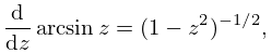
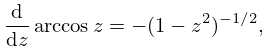
28: 4.24 Inverse Trigonometric Functions: Further Properties

… ►

§4.24(ii) Derivatives

►

4.24.7 $$\frac{d}{dz}\arcsin z={(1-z^2)}^{-1/2},$$

ⓘ

Symbols:

$\frac{df}{dx}$: derivative of $f$ with respect to $x$ , $\arcsin z$: arcsine function and $z$: complex variable

A&S Ref:

4.4.52

Permalink:

http://dlmf.nist.gov/4.24.E7

Encodings:

pMML, png, TeX

See also:

Annotations for §4.24(ii), §4.24 and Ch.4

►

4.24.8 $$\frac{d}{dz}\arccos z=-{(1-z^2)}^{-1/2},$$

ⓘ

Symbols:

$\frac{df}{dx}$: derivative of $f$ with respect to $x$ , $\arccos z$: arccosine function and $z$: complex variable

A&S Ref:

4.4.53

Permalink:

http://dlmf.nist.gov/4.24.E8

Encodings:

pMML, png, TeX

See also:

Annotations for §4.24(ii), §4.24 and Ch.4

►

4.24.9 $$\frac{d}{dz}\arctan z=\frac{1}{1+z^2}.$$

ⓘ

Symbols:

$\frac{df}{dx}$: derivative of $f$ with respect to $x$ , $\arctan z$: arctangent function and $z$: complex variable

A&S Ref:

4.4.54

Permalink:

http://dlmf.nist.gov/4.24.E9

Encodings:

pMML, png, TeX

See also:

Annotations for §4.24(ii), §4.24 and Ch.4

… ►

4.24.12 $$\frac{d}{dz}\mathrm{arccot}z=-\frac{1}{1+z^2}.$$

ⓘ

Symbols:

$\frac{df}{dx}$: derivative of $f$ with respect to $x$ , $\mathrm{arccot}z$: arccotangent function and $z$: complex variable

A&S Ref:

4.4.55

Permalink:

http://dlmf.nist.gov/4.24.E12

Encodings:

pMML, png, TeX

See also:

Annotations for §4.24(ii), §4.24 and Ch.4

…

29: 10.73 Physical Applications

… ►

10.73.1 $${\nabla }^{2}V=\frac{1}{r}\frac{\partial }{\partial r}\left(r\frac{\partial V}{\partial r}\right)+\frac{1}{r^2}\frac{{\partial }^{2}V}{{\partial \varphi }^2}+\frac{{\partial }^{2}V}{{\partial z}^2}=0,$$

ⓘ

Symbols:

$\frac{\partial f}{\partial x}$: partial derivative of $f$ with respect to $x$ and $\partial x$: partial differential of $x$

Permalink:

http://dlmf.nist.gov/10.73.E1

Encodings:

pMML, png, TeX

See also:

Annotations for §10.73(i), §10.73 and Ch.10

… ►

10.73.2 $${\nabla }^2\psi =\frac{1}{c^2}\frac{{\partial }^2\psi }{{\partial t}^2},$$

ⓘ

Symbols:

$\frac{\partial f}{\partial x}$: partial derivative of $f$ with respect to $x$ and $\partial x$: partial differential of $x$

Permalink:

http://dlmf.nist.gov/10.73.E2

Encodings:

pMML, png, TeX

See also:

Annotations for §10.73(i), §10.73 and Ch.10

… ►

10.73.3 $${\nabla }^{4}W+{\lambda }^2\frac{{\partial }^{2}W}{{\partial t}^2}=0.$$

ⓘ

Symbols:

$\frac{\partial f}{\partial x}$: partial derivative of $f$ with respect to $x$ and $\partial x$: partial differential of $x$

Permalink:

http://dlmf.nist.gov/10.73.E3

Encodings:

pMML, png, TeX

See also:

Annotations for §10.73(i), §10.73 and Ch.10

… ►

10.73.4 $$({\nabla }^2+k^2)f=\frac{1}{{\rho }^2}\frac{\partial }{\partial \rho }\left({\rho }^2\frac{\partial f}{\partial \rho }\right)+\frac{1}{{\rho }^2\sin \theta }\frac{\partial }{\partial \theta }\left(\sin \theta \frac{\partial f}{\partial \theta }\right)+\frac{1}{{\rho }^2{\sin }^2\theta }\frac{{\partial }^{2}f}{{\partial \varphi }^2}+k^{2}f.$$

ⓘ

Symbols:

$\frac{\partial f}{\partial x}$: partial derivative of $f$ with respect to $x$ , $\partial x$: partial differential of $x$ , $\sin z$: sine function and $k$: nonnegative integer

Permalink:

http://dlmf.nist.gov/10.73.E4

Encodings:

pMML, png, TeX

See also:

Annotations for §10.73(ii), §10.73 and Ch.10

…

30: 32.1 Special Notation

… ►Unless otherwise noted, primes indicate derivatives with respect to the argument. …