DLMF: Untitled Document

§26.21 Tables

►Abramowitz and Stegun (1964, Chapter 24) tabulates binomial coefficients

\genfrac{(}{)}{0.0pt}{}{m}{n}

for

m

up to 50 and

n

up to 25; extends Table 26.4.1 to

n=10

; tabulates Stirling numbers of the first and second kinds,

s\left(n,k\right)

and

S\left(n,k\right)

, for

n

up to 25 and

k

up to

n

; tabulates partitions

p\left(n\right)

and partitions into distinct parts

p\left(\mathcal{D},n\right)

for

n

up to 500. … ►It also contains a table of Gaussian polynomials up to

\genfrac{[}{]}{0.0pt}{}{12}{6}_{q}

. …

… ►

14.18.1

\mathsf{P}_{\nu}\left(\cos\theta_{1}\cos\theta_{2}+\sin\theta_{1}\sin\theta_{2% }\cos\phi\right)=\mathsf{P}_{\nu}\left(\cos\theta_{1}\right)\mathsf{P}_{\nu}% \left(\cos\theta_{2}\right)+2\sum_{m=1}^{\infty}(-1)^{m}\mathsf{P}^{-m}_{\nu}% \left(\cos\theta_{1}\right)\mathsf{P}^{m}_{\nu}\left(\cos\theta_{2}\right)\cos% \left(m\phi\right),

ⓘ

Symbols:: $\mathsf{P}^{\NVar{\mu}}_{\NVar{\nu}}\left(\NVar{x}\right)$ : Ferrers function of the first kind, $\cos\NVar{z}$ : cosine function, $\mathsf{P}_{\NVar{\nu}}\left(\NVar{x}\right)=\mathsf{P}^{0}_{\nu}\left(x\right)$ : Ferrers function of the first kind, $\sin\NVar{z}$ : sine function, $m$ : nonnegative integer, $\nu$ : general degree, $\theta_{1}$ , $\theta_{2}$ : real and $\phi$ : real
Referenced by:: §14.18(ii), §14.18(ii)
Permalink:: http://dlmf.nist.gov/14.18.E1
Encodings:: pMML, png, TeX
See also:: Annotations for §14.18(ii), §14.18 and Ch.14

►

14.18.2

\mathsf{P}_{n}\left(\cos\theta_{1}\cos\theta_{2}+\sin\theta_{1}\sin\theta_{2}% \cos\phi\right)=\sum_{m=-n}^{n}(-1)^{m}\mathsf{P}^{-m}_{n}\left(\cos\theta_{1}% \right)\mathsf{P}^{m}_{n}\left(\cos\theta_{2}\right)\cos\left(m\phi\right).

ⓘ

Symbols:: $\mathsf{P}^{\NVar{\mu}}_{\NVar{\nu}}\left(\NVar{x}\right)$ : Ferrers function of the first kind, $\cos\NVar{z}$ : cosine function, $\mathsf{P}_{\NVar{\nu}}\left(\NVar{x}\right)=\mathsf{P}^{0}_{\nu}\left(x\right)$ : Ferrers function of the first kind, $\sin\NVar{z}$ : sine function, $m$ : nonnegative integer, $n$ : nonnegative integer, $\theta_{1}$ , $\theta_{2}$ : real and $\phi$ : real
Referenced by:: §14.18(ii), §14.18(ii)
Permalink:: http://dlmf.nist.gov/14.18.E2
Encodings:: pMML, png, TeX
See also:: Annotations for §14.18(ii), §14.18 and Ch.14

… ►

14.18.3

\mathsf{Q}_{\nu}\left(\cos\theta_{1}\cos\theta_{2}+\sin\theta_{1}\sin\theta_{2% }\cos\phi\right)=\mathsf{P}_{\nu}\left(\cos\theta_{1}\right)\mathsf{Q}_{\nu}% \left(\cos\theta_{2}\right)+2\sum_{m=1}^{\infty}(-1)^{m}\mathsf{P}^{-m}_{\nu}% \left(\cos\theta_{1}\right)\mathsf{Q}^{m}_{\nu}\left(\cos\theta_{2}\right)\cos% \left(m\phi\right).

ⓘ

Symbols:: $\mathsf{P}^{\NVar{\mu}}_{\NVar{\nu}}\left(\NVar{x}\right)$ : Ferrers function of the first kind, $\mathsf{Q}^{\NVar{\mu}}_{\NVar{\nu}}\left(\NVar{x}\right)$ : Ferrers function of the second kind, $\cos\NVar{z}$ : cosine function, $\mathsf{P}_{\NVar{\nu}}\left(\NVar{x}\right)=\mathsf{P}^{0}_{\nu}\left(x\right)$ : Ferrers function of the first kind, $\mathsf{Q}_{\NVar{\nu}}\left(\NVar{x}\right)=\mathsf{Q}^{0}_{\nu}\left(x\right)$ : Ferrers function of the second kind, $\sin\NVar{z}$ : sine function, $m$ : nonnegative integer, $\nu$ : general degree, $\theta_{1}$ , $\theta_{2}$ : real and $\phi$ : real
Referenced by:: §14.18(ii), Ch.14
Permalink:: http://dlmf.nist.gov/14.18.E3
Encodings:: pMML, png, TeX
See also:: Annotations for §14.18(ii), §14.18 and Ch.14

… ►

14.18.6

(x-y)\sum_{k=0}^{n}(2k+1)P_{k}\left(x\right)P_{k}\left(y\right)=(n+1)\left(P_{% n+1}\left(x\right)P_{n}\left(y\right)-P_{n}\left(x\right)P_{n+1}\left(y\right)% \right),

ⓘ

Symbols:: $P_{\NVar{\nu}}\left(\NVar{z}\right)=P^{0}_{\nu}\left(z\right)$ : Legendre function of the first kind and $n$ : nonnegative integer
A&S Ref:: 8.9.1
Referenced by:: Erratum (V1.0.7) for Subsection 14.18(iii)
Permalink:: http://dlmf.nist.gov/14.18.E6
Encodings:: pMML, png, TeX
See also:: Annotations for §14.18(iii), §14.18(iii), §14.18 and Ch.14

►

14.18.7

(x-y)\sum_{k=0}^{n}(2k+1)P_{k}\left(x\right)Q_{k}\left(y\right)=(n+1)\left(P_{% n+1}\left(x\right)Q_{n}\left(y\right)-P_{n}\left(x\right)Q_{n+1}\left(y\right)% \right)-1.

ⓘ

Symbols:: $P_{\NVar{\nu}}\left(\NVar{z}\right)=P^{0}_{\nu}\left(z\right)$ : Legendre function of the first kind, $Q_{\NVar{\nu}}\left(\NVar{z}\right)=Q^{0}_{\nu}\left(z\right)$ : Legendre function of the second kind and $n$ : nonnegative integer
A&S Ref:: 8.9.2
Referenced by:: §14.18(iii), Erratum (V1.0.7) for Subsection 14.18(iii)
Permalink:: http://dlmf.nist.gov/14.18.E7
Encodings:: pMML, png, TeX
See also:: Annotations for §14.18(iii), §14.18(iii), §14.18 and Ch.14

…

… ►

§14.9(i) Connections Between $\mathsf{P}^{\pm\mu}_{\nu}\left(x\right)$ , $\mathsf{P}^{\pm\mu}_{-\nu-1}\left(x\right)$ , $\mathsf{Q}^{\pm\mu}_{\nu}\left(x\right)$ , $\mathsf{Q}^{\mu}_{-\nu-1}\left(x\right)$

… ►

\mathsf{P}^{\mu}_{-\nu-1}\left(x\right)=\mathsf{P}^{\mu}_{\nu}\left(x\right),

►

\mathsf{P}^{-\mu}_{-\nu-1}\left(x\right)=\mathsf{P}^{-\mu}_{\nu}\left(x\right),

… ►

§14.9(ii) Connections Between $\mathsf{P}^{\pm\mu}_{\nu}\left(\pm x\right)$ , $\mathsf{Q}^{-\mu}_{\nu}\left(\pm x\right)$ , $\mathsf{Q}^{\mu}_{\nu}\left(x\right)$

… ►

§14.9(iii) Connections Between $P^{\pm\mu}_{\nu}\left(x\right)$ , $P^{\pm\mu}_{-\nu-1}\left(x\right)$ , $\boldsymbol{Q}^{\pm\mu}_{\nu}\left(x\right)$ , $\boldsymbol{Q}^{\mu}_{-\nu-1}\left(x\right)$

…

… ►

29.17.1

F(z)=E(z)\int_{\mathrm{i}{K^{\prime}}}^{z}\frac{\,\mathrm{d}u}{(E(u))^{2}}.

ⓘ

Symbols:: ${K^{\prime}}\left(\NVar{k}\right)$ : Legendre’s complementary complete elliptic integral of the first kind, $\,\mathrm{d}\NVar{x}$ : differential of $x$ , $\mathrm{i}$ : imaginary unit, $\int$ : integral, $z$ : complex variable and $k$ : real parameter
Permalink:: http://dlmf.nist.gov/29.17.E1
Encodings:: pMML, png, TeX
See also:: Annotations for §29.17(i), §29.17 and Ch.29

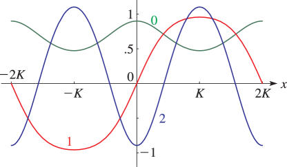
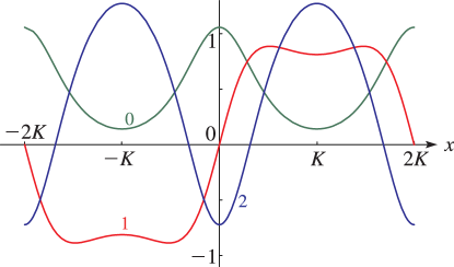
… ►They are algebraic functions of

\operatorname{sn}\left(z,k\right)

,

\operatorname{cn}\left(z,k\right)

, and

\operatorname{dn}\left(z,k\right)

, and have primitive period

8K

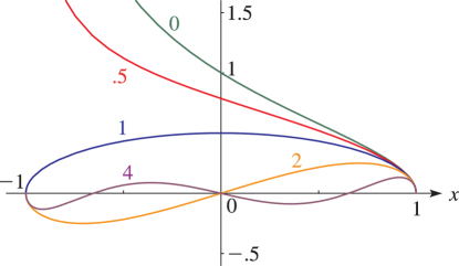
. … ►Lamé–Wangerin functions are solutions of (29.2.1) with the property that

(\operatorname{sn}\left(z,k\right))^{1/2}w(z)

is bounded on the line segment from

\mathrm{i}{K^{\prime}}

to

2K+\mathrm{i}{K^{\prime}}

. …

… ►

See accompanying text — Figure 14.4.1: $\mathsf{P}^{0}_{\nu}\left(x\right)$ , $\nu=0,\tfrac{1}{2},1,2,4$ . Magnify

►

…

… ►

•

Abramowitz and Stegun (1964, Chapter 8) tabulates $\mathsf{P}_{n}\left(x\right)$ for $n=0(1)3,9,10$ , $x=0(.01)1$ , 5–8D; $\mathsf{P}_{n}'\left(x\right)$ for $n=1(1)4,9,10$ , $x=0(.01)1$ , 5–7D; $\mathsf{Q}_{n}\left(x\right)$ and $\mathsf{Q}_{n}'\left(x\right)$ for $n=0(1)3,9,10$ , $x=0(.01)1$ , 6–8D; $P_{n}\left(x\right)$ and $P_{n}'\left(x\right)$ for $n=0(1)5,9,10$ , $x=1(.2)10$ , 6S; $Q_{n}\left(x\right)$ and $Q_{n}'\left(x\right)$ for $n=0(1)3,9,10$ , $x=1(.2)10$ , 6S. (Here primes denote derivatives with respect to $x$ .)

►

•

Zhang and Jin (1996, Chapter 4) tabulates $\mathsf{P}_{n}\left(x\right)$ for $n=2(1)5,10$ , $x=0(.1)1$ , 7D; $\mathsf{P}_{n}\left(\cos\theta\right)$ for $n=1(1)4,10$ , $\theta=0(5^{\circ})90^{\circ}$ , 8D; $\mathsf{Q}_{n}\left(x\right)$ for $n=0(1)2,10$ , $x=0(.1)0.9$ , 8S; $\mathsf{Q}_{n}\left(\cos\theta\right)$ for $n=0(1)3,10$ , $\theta=0(5^{\circ})90^{\circ}$ , 8D; $\mathsf{P}^{m}_{n}\left(x\right)$ for $m=1(1)4$ , $n-m=0(1)2$ , $n=10$ , $x=0,0.5$ , 8S; $\mathsf{Q}^{m}_{n}\left(x\right)$ for $m=1(1)4$ , $n=0(1)2,10$ , 8S; $\mathsf{P}^{m}_{\nu}\left(\cos\theta\right)$ for $m=0(1)3$ , $\nu=0(.25)5$ , $\theta=0(15^{\circ})90^{\circ}$ , 5D; $P_{n}\left(x\right)$ for $n=2(1)5,10$ , $x=1(1)10$ , 7S; $Q_{n}\left(x\right)$ for $n=0(1)2,10$ , $x=2(1)10$ , 8S. Corresponding values of the derivative of each function are also included, as are 6D values of the first 5 $\nu$ -zeros of $\mathsf{P}^{m}_{\nu}\left(\cos\theta\right)$ and of its derivative for $m=0(1)4$ , $\theta=10^{\circ},30^{\circ},150^{\circ}$ .

►

•

Belousov (1962) tabulates $\mathsf{P}^{m}_{n}\left(\cos\theta\right)$ (normalized) for $m=0(1)36$ , $n-m=0(1)56$ , $\theta=0(2.5^{\circ})90^{\circ}$ , 6D.

►

•

Žurina and Karmazina (1964, 1965) tabulate the conical functions $\mathsf{P}_{-\frac{1}{2}+\mathrm{i}\tau}\left(x\right)$ for $\tau=0(.01)50$ , $x=-0.9(.1)0.9$ , 7S; $P_{-\frac{1}{2}+\mathrm{i}\tau}\left(x\right)$ for $\tau=0(.01)50$ , $x=1.1(.1)2(.2)5(.5)10(10)60$ , 7D. Auxiliary tables are included to facilitate computation for larger values of $\tau$ when $-1<x<1$ .

►

•

Žurina and Karmazina (1963) tabulates the conical functions $\mathsf{P}^{1}_{-\frac{1}{2}+\mathrm{i}\tau}\left(x\right)$ for $\tau=0(.01)25$ , $x=-0.9(.1)0.9$ , 7S; $P^{1}_{-\frac{1}{2}+\mathrm{i}\tau}\left(x\right)$ for $\tau=0(.01)25$ , $x=1.1(.1)2(.2)5(.5)10(10)60$ , 7S. Auxiliary tables are included to assist computation for larger values of $\tau$ when $-1<x<1$ .

…