finite sum
(0.002 seconds)
31—40 of 75 matching pages
31: 8.11 Asymptotic Approximations and Expansions
…
►
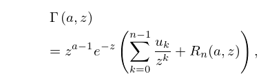
8.11.2
.
…
►
8.11.4
.
►This expansion is absolutely convergent for all finite
, and it can also be regarded as a generalized asymptotic expansion (§2.1(v)) of as in .
…
►
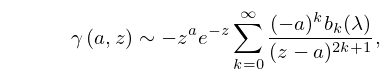
8.11.6
, .
…
►
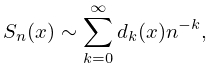
8.11.18
,
…
32: 1.18 Linear Second Order Differential Operators and Eigenfunction Expansions
…
►A (finite or countably infinite, generalizing the definition of (1.2.40)) set is an orthonormal set if the are normalized and pairwise orthogonal.
…
►where the infinite sum means convergence in norm,
…
►If is finite then is bounded, and extends uniquely to a bounded linear operator on .
…
►Consider the second order differential operator acting on real functions of in the finite interval
…
►Let be a finite or infinite open interval in .
…
33: 33.6 Power-Series Expansions in
…
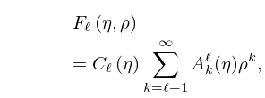
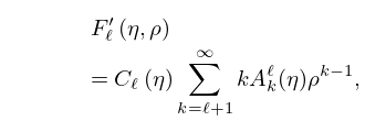
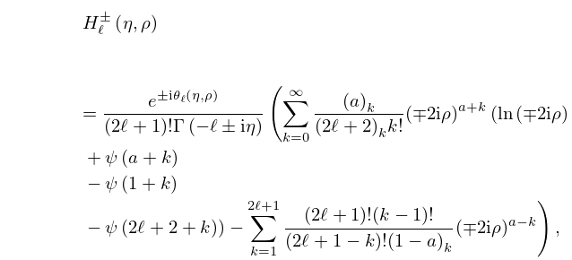
►
33.6.1
►
33.6.2
…
►
33.6.5
…
►The series (33.6.1), (33.6.2), and (33.6.5) converge for all finite values of .
…
34: 1.10 Functions of a Complex Variable
…
►Next, is a pole if for at least one, but only finitely many, negative .
…
►If is analytic within a simple closed contour , and continuous within and on —except in both instances for a finite number of singularities within —then
…
►A cut domain is one from which the points on finitely many nonintersecting simple contours (§1.9(iii)) have been removed.
…
►Let be a domain and be a closed finite segment of the real axis.
…
►(The integer may be greater than one to allow for a finite number of zero factors.)
…
35: 18.39 Applications in the Physical Sciences
…
►where is a spatial coordinate, the mass of the particle with potential energy , is the reduced Planck’s constant, and a finite or infinite interval.
…
►As in classical dynamics this sum is the total energy of the one particle system.
…
►The finite system of functions is orthonormal in , see (18.34.7_3).
…
►The fact that both the eigenvalues of (18.39.31) and the scaling of the co-ordinate in the eigenfunctions, (18.39.30), depend on the sum
leads to the substitution
…
►This equivalent quadrature relationship, see Heller et al. (1973), Yamani and Reinhardt (1975), allows extraction of scattering information from the finite dimensional functions of (18.39.53), provided that such information involves potentials, or projections onto functions, exactly expressed, or well approximated, in the finite basis of (18.39.44).
…
36: 23.20 Mathematical Applications
…
►Let denote the set of points on that are of finite order (that is, those points for which there exists a positive integer with ), and let be the sets of points with integer and rational coordinates, respectively.
…Both and are finite sets.
…To determine , we make use of the fact that if then must be a divisor of ; hence there are only a finite number of possibilities for .
…The resulting points are then tested for finite order as follows.
…If any of these quantities is zero, then the point has finite order.
…
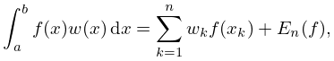
37: 3.5 Quadrature
…
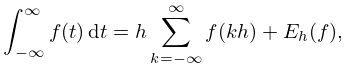
►
3.5.5
…
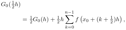
►
3.5.12
…
►
3.5.15
…
►Let denote the set of monic polynomials of degree (coefficient of equal to ) that are orthogonal with respect to a positive weight function on a finite or infinite interval ; compare §18.2(i).
…In particular, with , we have a finite system of orthogonal polynomials () on with respect to the weights :
…
38: 1.4 Calculus of One Variable
…
►If is continuous on an interval save for a finite number of simple discontinuities, then is piecewise (or sectionally) continuous on .
…
►For nondecreasing on the closure of an interval , the measure is absolutely continuous if is continuous and there exists a weight function
, Riemann (or Lebesgue) integrable on finite subintervals of , such that
…
►Similarly, assume that exists for all finite values of (), but not necessarily when .
…
►With , the total variation of on a finite or infinite interval is
…
►Lastly, whether or not the real numbers and satisfy , and whether or not they are finite, we define
by (1.4.34) whenever this integral exists.
…
39: 15.17 Mathematical Applications
…
►In combinatorics, hypergeometric identities classify single sums of products of binomial coefficients.
…
►These monodromy groups are finite iff the solutions of Riemann’s differential equation are all algebraic.
…
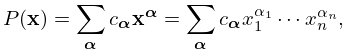
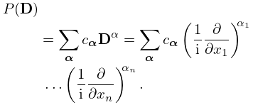
40: 1.16 Distributions
…
►A sequence of functions in is said to converge to a function as if the sequence converges uniformly to on every finite interval and if the constants in the inequalities
…
►
1.16.31
…
►
1.16.32
►Here ranges over a finite set of multi-indices, is a multivariate polynomial, and is a partial differential operator.
…
