eigenvalues

SearchAdvancedHelp

(0.001 seconds)

31—40 of 87 matching pages

31: 29.1 Special Notation

… ►All derivatives are denoted by differentials, not by primes. ►The main functions treated in this chapter are the eigenvalues $a_{\nu }^{2m}\left(k^2\right)$, $a_{\nu }^{2m+1}\left(k^2\right)$, $b_{\nu }^{2m+1}\left(k^2\right)$, $b_{\nu }^{2m+2}\left(k^2\right)$, the Lamé functions ${\mathrm{𝐸𝑐}}_{\nu }^{2m}(z,k^2)$, ${\mathrm{𝐸𝑐}}_{\nu }^{2m+1}(z,k^2)$, ${\mathrm{𝐸𝑠}}_{\nu }^{2m+1}(z,k^2)$, ${\mathrm{𝐸𝑠}}_{\nu }^{2m+2}(z,k^2)$, and the Lamé polynomials ${\mathrm{𝑢𝐸}}_{2n}^m(z,k^2)$, ${\mathrm{𝑠𝐸}}_{2n+1}^m(z,k^2)$, ${\mathrm{𝑐𝐸}}_{2n+1}^m(z,k^2)$, ${\mathrm{𝑑𝐸}}_{2n+1}^m(z,k^2)$, ${\mathrm{𝑠𝑐𝐸}}_{2n+2}^m(z,k^2)$, ${\mathrm{𝑠𝑑𝐸}}_{2n+2}^m(z,k^2)$, ${\mathrm{𝑐𝑑𝐸}}_{2n+2}^m(z,k^2)$, ${\mathrm{𝑠𝑐𝑑𝐸}}_{2n+3}^m(z,k^2)$. The notation for the eigenvalues and functions is due to Erdélyi et al. (1955, §15.5.1) and that for the polynomials is due to Arscott (1964b, §9.3.2). … ►Other notations that have been used are as follows: Ince (1940a) interchanges $a_{\nu }^{2m+1}\left(k^2\right)$ with $b_{\nu }^{2m+1}\left(k^2\right)$. … ►

$${(s_{\nu }^m(k^2))}^2=\frac{4}{\pi }{\int }_0^K{\left({\mathrm{𝐸𝑠}}_{\nu }^m(x,k^2)\right)}^{2}dx.$$

32: 30.9 Asymptotic Approximations and Expansions

§30.9 Asymptotic Approximations and Expansions

… ►

30.9.1 $${\lambda }_n^m\left({\gamma }^2\right)\sim -{\gamma }^2+\gamma q+{\beta }_0+{\beta }_1{\gamma }^{-1}+{\beta }_2{\gamma }^{-2}+\mathrm{\cdots },$$

ⓘ

Symbols:

$\sim$: Poincaré asymptotic expansion, ${\lambda }_n^m\left({\gamma }^2\right)$: eigenvalues of the spheroidal differential equation, $m$: nonnegative integer, $n\ge m$: integer degree, ${\gamma }^2$: real parameter, $q$ and ${\beta }_n$: coeffients

A&S Ref:

21.7.6

Referenced by:

item

Permalink:

http://dlmf.nist.gov/30.9.E1

Encodings:

pMML, png, TeX

See also:

Annotations for §30.9(i), §30.9 and Ch.30

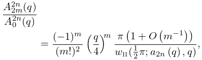
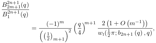
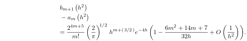
… ►The asymptotic behavior of ${\lambda }_n^m\left({\gamma }^2\right)$ and $a_{n,k}^m({\gamma }^2)$ as $n\to \mathrm{\infty }$ in descending powers of $2n+1$ is derived in Meixner (1944). …The behavior of ${\lambda }_n^m\left({\gamma }^2\right)$ for complex ${\gamma }^2$ and large $|{\lambda }_n^m\left({\gamma }^2\right)|$ is investigated in Hunter and Guerrieri (1982).

33: 30.7 Graphics

… ►

§30.7(i) Eigenvalues

►

►►

Figure 30.7.1: Eigenvalues ${\lambda }_n^0\left({\gamma }^2\right)$, $n=0,1,2,3$, $-10\le {\gamma }^2\le 10$. Magnify

►

►►

Figure 30.7.2: Eigenvalues ${\lambda }_n^1\left({\gamma }^2\right)$ $n=1,2,3,4$, $-10\le {\gamma }^2\le 10$. Magnify

►

►►

Figure 30.7.3: Eigenvalues ${\lambda }_n^5\left({\gamma }^2\right)$, $n=5,6,7,8$, $-40\le {\gamma }^2\le 40$. Magnify

►

►►

Figure 30.7.4: Eigenvalues ${\lambda }_n^{10}\left({\gamma }^2\right)$, $n=10,11,12,13$, $-50\le {\gamma }^2\le 150$. Magnify

…

34: 28.4 Fourier Series

… ►

$(a-4m^2)A_{2m}-q(A_{2m-2}+A_{2m+2})=0$ , $m=2,3,4,\mathrm{\dots }$, $a=a_{2n}\left(q\right)$, $A_{2m}=A_{2m}^{2n}(q)$.

… ►

28.4.24 $$\frac{A_{2m}^{2n}(q)}{A_0^{2n}(q)}=\frac{{(-1)}^m}{{(m!)}^2}{\left(\frac{q}{4}\right)}^m\frac{\pi \left(1+O\left(m^{-1}\right)\right)}{w_{\text{II}}(\frac{1}{2}\pi ;a_{2n}\left(q\right),q)},$$

ⓘ

Symbols:

$O\left(x\right)$: order not exceeding, $a_n\left(q\right)$: eigenvalues of Mathieu equation, $\pi$: the ratio of the circumference of a circle to its diameter, $!$: factorial (as in $n!$), $m$: integer, $q=h^2$: parameter, $n$: integer, $w_{\text{II}}(z;a,q)$: fundamental solution and $A_m(q)$: Fourier coefficient

Permalink:

http://dlmf.nist.gov/28.4.E24

Encodings:

pMML, png, TeX

See also:

Annotations for §28.4(vii), §28.4 and Ch.28

►

28.4.25 $$\frac{A_{2m+1}^{2n+1}(q)}{A_1^{2n+1}(q)}=\frac{{(-1)}^{m+1}}{{\left({\left(\frac{1}{2}\right)}_{m+1}\right)}^2}{\left(\frac{q}{4}\right)}^{m+1}\frac{2\left(1+O\left(m^{-1}\right)\right)}{w_{\text{II}}^{\prime }(\frac{1}{2}\pi ;a_{2n+1}\left(q\right),q)},$$

ⓘ

Symbols:

$O\left(x\right)$: order not exceeding, $a_n\left(q\right)$: eigenvalues of Mathieu equation, ${\left(a\right)}_n$: Pochhammer’s symbol (or shifted factorial), $\pi$: the ratio of the circumference of a circle to its diameter, $m$: integer, $q=h^2$: parameter, $n$: integer, $w(z)$: Mathieu’s equation solution and $A_m(q)$: Fourier coefficient

Permalink:

http://dlmf.nist.gov/28.4.E25

Encodings:

pMML, png, TeX

See also:

Annotations for §28.4(vii), §28.4 and Ch.28

►

28.4.26 $$\frac{B_{2m+1}^{2n+1}(q)}{B_1^{2n+1}(q)}=\frac{{(-1)}^m}{{\left({\left(\frac{1}{2}\right)}_{m+1}\right)}^2}{\left(\frac{q}{4}\right)}^{m+1}\frac{2\left(1+O\left(m^{-1}\right)\right)}{w_{\text{I}}(\frac{1}{2}\pi ;b_{2n+1}\left(q\right),q)},$$

ⓘ

Symbols:

$O\left(x\right)$: order not exceeding, $b_n\left(q\right)$: eigenvalues of Mathieu equation, ${\left(a\right)}_n$: Pochhammer’s symbol (or shifted factorial), $\pi$: the ratio of the circumference of a circle to its diameter, $m$: integer, $q=h^2$: parameter, $n$: integer, $w_{\text{I}}(z;a,q)$: fundamental solution and $B_m(q)$: Fourier coefficient

Permalink:

http://dlmf.nist.gov/28.4.E26

Encodings:

pMML, png, TeX

See also:

Annotations for §28.4(vii), §28.4 and Ch.28

►

28.4.27 $$\frac{B_{2m}^{2n+2}(q)}{B_2^{2n+2}(q)}=\frac{{(-1)}^m}{{(m!)}^2}{\left(\frac{q}{4}\right)}^m\frac{q\pi \left(1+O\left(m^{-1}\right)\right)}{w_{\text{I}}^{\prime }(\frac{1}{2}\pi ;b_{2n+2}\left(q\right),q)}.$$

ⓘ

Symbols:

$O\left(x\right)$: order not exceeding, $b_n\left(q\right)$: eigenvalues of Mathieu equation, $\pi$: the ratio of the circumference of a circle to its diameter, $!$: factorial (as in $n!$), $m$: integer, $q=h^2$: parameter, $n$: integer, $w(z)$: Mathieu’s equation solution and $B_m(q)$: Fourier coefficient

Permalink:

http://dlmf.nist.gov/28.4.E27

Encodings:

pMML, png, TeX

See also:

Annotations for §28.4(vii), §28.4 and Ch.28

…

35: 28.29 Definitions and Basic Properties

… ►iff ${\mathrm{e}}^{\pi \mathrm{i}\nu }$ is an eigenvalue of the matrix … ►

§28.29(iii) Discriminant and Eigenvalues in the Real Case

… ►To every equation (28.29.1), there belong two increasing infinite sequences of real eigenvalues: ►

28.29.16 $${\lambda }_n,n=0,1,2,\mathrm{\dots },\text{ with }△({\lambda }_n)=2,$$

ⓘ

Defines:

${\lambda }_n$: eigenvalues (locally)

Symbols:

$n$: integer

Referenced by:

§28.30(i)

Permalink:

http://dlmf.nist.gov/28.29.E16

Encodings:

pMML, png, TeX

See also:

Annotations for §28.29(iii), §28.29 and Ch.28

►

28.29.17 $${\mu }_n,n=1,2,3,\mathrm{\dots },\text{ with }△({\mu }_n)=-2.$$

ⓘ

Defines:

${\mu }_n$: eigenvalues (locally)

Symbols:

$n$: integer

Referenced by:

§28.30(i)

Permalink:

http://dlmf.nist.gov/28.29.E17

Encodings:

pMML, png, TeX

See also:

Annotations for §28.29(iii), §28.29 and Ch.28

…

36: Hans Volkmer

… ►His book Multiparameter Eigenvalue Problems and Expansion Theorems was published by Springer as Lecture Notes in Mathematics No. …

37: 3.7 Ordinary Differential Equations

… ►

§3.7(iv) Sturm–Liouville Eigenvalue Problems

… ►The Sturm–Liouville eigenvalue problem is the construction of a nontrivial solution of the system …The values ${\lambda }_k$ are the eigenvalues and the corresponding solutions $w_k$ of the differential equation are the eigenfunctions. The eigenvalues ${\lambda }_k$ are simple, that is, there is only one corresponding eigenfunction (apart from a normalization factor), and when ordered increasingly the eigenvalues satisfy … ►The larger the absolute values of the eigenvalues ${\lambda }_k$ that are being sought, the smaller the integration steps $\left|{\tau }_j\right|$ need to be. …

38: 28.8 Asymptotic Expansions for Large $q$

§28.8 Asymptotic Expansions for Large $q$

►

§28.8(i) Eigenvalues

… ►

28.8.1 $$\begin{array}{c}{a}_m\left(h^2\right)\\ b_{m+1}\left(h^2\right)\end{array}\}\sim -2h^2+2sh-\frac{1}{8}(s^2+1)-\frac{1}{2^{7}h}(s^3+3s)-\frac{1}{2^{12}{h}^2}(5s^4+34s^2+9)-\frac{1}{2^{17}{h}^3}(33s^5+410s^3+405s)-\frac{1}{2^{20}{h}^4}(63s^6+1260s^4+2943s^2+486)-\frac{1}{2^{25}{h}^5}(527s^7+15617s^5+69001s^3+41607s)+\mathrm{\cdots }.$$

ⓘ

Symbols:

$a_n\left(q\right)$: eigenvalues of Mathieu equation, $b_n\left(q\right)$: eigenvalues of Mathieu equation, $\sim$: Poincaré asymptotic expansion, $m$: integer and $h$: parameter

A&S Ref:

20.2.30 (in different form)

Referenced by:

§28.8(i), Erratum (V1.1.10) for Sections 28.6(i), 28.6(ii), 28.8(i), 28.8(ii)

Permalink:

http://dlmf.nist.gov/28.8.E1

Encodings:

pMML, png, TeX

See also:

Annotations for §28.8(i), §28.8 and Ch.28

… ►

28.8.2 $$b_{m+1}\left(h^2\right)-a_m\left(h^2\right)=\frac{2^{4m+5}}{m!}{\left(\frac{2}{\pi }\right)}^{1/2}{h}^{m+(3/2)}{\mathrm{e}}^{-4h}\left(1-\frac{6m^2+14m+7}{32h}+O\left(\frac{1}{h^2}\right)\right).$$

ⓘ

Symbols:

$O\left(x\right)$: order not exceeding, $a_n\left(q\right)$: eigenvalues of Mathieu equation, $b_n\left(q\right)$: eigenvalues of Mathieu equation, $\pi$: the ratio of the circumference of a circle to its diameter, $\mathrm{e}$: base of natural logarithm, $!$: factorial (as in $n!$), $m$: integer and $h$: parameter

A&S Ref:

20.2.31

Permalink:

http://dlmf.nist.gov/28.8.E2

Encodings:

pMML, png, TeX

See also:

Annotations for §28.8(i), §28.8 and Ch.28

…

39: 19.31 Probability Distributions

… ►More generally, let $𝐀$ ($=[a_{r,s}]$) and $𝐁$ ($=[b_{r,s}]$) be real positive-definite matrices with $n$ rows and $n$ columns, and let ${\lambda }_1,\mathrm{\dots },{\lambda }_n$ be the eigenvalues of $𝐀{𝐁}^{-1}$. … ►

19.31.2 $${\int }_{{ℝ}^n}{({𝐱}^{\mathrm{T}}𝐀𝐱)}^{\mu }\exp \left(-{𝐱}^{\mathrm{T}}𝐁𝐱\right)d{x}_1\mathrm{\cdots }d{x}_n=\frac{{\pi }^{n/2}\mathrm{\Gamma }\left(\mu +\frac{1}{2}n\right)}{\sqrt{det𝐁}\mathrm{\Gamma }\left(\frac{1}{2}n\right)}{R}_{\mu }(\frac{1}{2},\mathrm{\dots },\frac{1}{2};{\lambda }_1,\mathrm{\dots },{\lambda }_n),$$ $\mu >-\frac{1}{2}n$.

ⓘ

Symbols:

$R_{-a}(b_1,\mathrm{\dots },b_n;z_1,\mathrm{\dots },z_n)$ or $R_{-a}(𝐛;𝐳)$: multivariate hypergeometric function, $\mathrm{\Gamma }\left(z\right)$: gamma function, $\pi$: the ratio of the circumference of a circle to its diameter, $det$: determinant, $dx$: differential of $x$ , $\exp z$: exponential function, $\int$: integral, $ℝ$: real line, ${𝐀}^{\mathrm{T}}$: transpose of matrix, $n$: nonnegative integer and ${\lambda }_n$: eigenvalues

Referenced by:

§19.31

Permalink:

http://dlmf.nist.gov/19.31.E2

Encodings:

pMML, png, TeX

See also:

Annotations for §19.31 and Ch.19

…

40: 32.14 Combinatorics

… ►The distribution function $F(s)$ given by (32.14.2) arises in random matrix theory where it gives the limiting distribution for the normalized largest eigenvalue in the Gaussian Unitary Ensemble of $n\times n$ Hermitian matrices; see Tracy and Widom (1994). …