doxycycline pills black market 365-RX.com/?id=1738

SearchAdvancedHelp

Did you mean cyclice mills black market 365-becom/?id=1738 ?

(0.052 seconds)

1—10 of 30 matching pages

1: 14.24 Analytic Continuation

… ►Let $s$ be an arbitrary integer, and $P_{\nu }^{-\mu }\left(z{\mathrm{e}}^{s\pi \mathrm{i}}\right)$ and ${𝑸}_{\nu }^{\mu }\left(z{\mathrm{e}}^{s\pi \mathrm{i}}\right)$ denote the branches obtained from the principal branches by making $\frac{1}{2}s$ circuits, in the positive sense, of the ellipse having $\pm 1$ as foci and passing through $z$. … ►

14.24.2 $${𝑸}_{\nu }^{\mu }\left(z{\mathrm{e}}^{s\pi \mathrm{i}}\right)={(-1)}^s{\mathrm{e}}^{-s\nu \pi \mathrm{i}}{𝑸}_{\nu }^{\mu }\left(z\right),$$

ⓘ

Symbols:

${𝑸}_{\nu }^{\mu }\left(z\right)$: Olver’s associated Legendre function, $\pi$: the ratio of the circumference of a circle to its diameter, $\mathrm{e}$: base of natural logarithm, $\mathrm{i}$: imaginary unit, $z$: complex variable, $\mu$: general order, $\nu$: general degree and $s$: arbitrary integer

Referenced by:

§14.23, §14.24

Permalink:

http://dlmf.nist.gov/14.24.E2

Encodings:

pMML, png, TeX

See also:

Annotations for §14.24 and Ch.14

… ►Next, let $P_{\nu ,s}^{-\mu }\left(z\right)$ and ${𝑸}_{\nu ,s}^{\mu }\left(z\right)$ denote the branches obtained from the principal branches by encircling the branch point $1$ (but not the branch point $-1$) $s$ times in the positive sense. … ►For fixed $z$, other than $\pm 1$ or $\mathrm{\infty }$, each branch of $P_{\nu }^{-\mu }\left(z\right)$ and ${𝑸}_{\nu }^{\mu }\left(z\right)$ is an entire function of each parameter $\nu$ and $\mu$. ►The behavior of $P_{\nu }^{-\mu }\left(z\right)$ and ${𝑸}_{\nu }^{\mu }\left(z\right)$ as $z\to -1$ from the left on the upper or lower side of the cut from $-\mathrm{\infty }$ to $1$ can be deduced from (14.8.7)–(14.8.11), combined with (14.24.1) and (14.24.2) with $s=\pm 1$.

2: 14.4 Graphics

… ►

►►

Figure 14.4.18: ${𝑸}_{\nu }^0\left(x\right)$, $\nu =0,\frac{1}{2},1,2,4$. Magnify

… ►

►►

Figure 14.4.20: ${𝑸}_{\nu }^{1/2}\left(x\right)$, $\nu =0,\frac{1}{2},1,2,4$. Magnify

… ►

►►

Figure 14.4.22: ${𝑸}_{\nu }^1\left(x\right)$, $\nu =0,\frac{1}{2},1,2,4$. Magnify

… ►

►►

Figure 14.4.24: ${𝑸}_0^{\mu }\left(x\right)$, $\mu =0,2,4,8$. Magnify

… ►

►►

Figure 14.4.28: ${𝑸}_1^{\mu }\left(x\right)$, $\mu =0,2,4,8$. Magnify

…

3: 14.21 Definitions and Basic Properties

… ►Standard solutions: the associated Legendre functions $P_{\nu }^{\mu }\left(z\right)$, $P_{\nu }^{-\mu }\left(z\right)$, ${𝑸}_{\nu }^{\mu }\left(z\right)$, and ${𝑸}_{-\nu -1}^{\mu }\left(z\right)$. $P_{\nu }^{\pm \mu }\left(z\right)$ and ${𝑸}_{\nu }^{\mu }\left(z\right)$ exist for all values of $\nu$, $\mu$, and $z$, except possibly $z=\pm 1$ and $\mathrm{\infty }$, which are branch points (or poles) of the functions, in general. When $z$ is complex $P_{\nu }^{\pm \mu }\left(z\right)$, $Q_{\nu }^{\mu }\left(z\right)$, and ${𝑸}_{\nu }^{\mu }\left(z\right)$ are defined by (14.3.6)–(14.3.10) with $x$ replaced by $z$: the principal branches are obtained by taking the principal values of all the multivalued functions appearing in these representations when $z\in (1,\mathrm{\infty })$, and by continuity elsewhere in the $z$-plane with a cut along the interval $(-\mathrm{\infty },1]$; compare §4.2(i). The principal branches of $P_{\nu }^{\pm \mu }\left(z\right)$ and ${𝑸}_{\nu }^{\mu }\left(z\right)$ are real when $\nu$, $\mu \in ℝ$ and $z\in (1,\mathrm{\infty })$. … ►When $\mathrm{\Re }\nu \ge -\frac{1}{2}$ and $\mathrm{\Re }\mu \ge 0$, a numerically satisfactory pair of solutions of (14.21.1) in the half-plane $|\mathrm{ph}z|\le \frac{1}{2}\pi$ is given by $P_{\nu }^{-\mu }\left(z\right)$ and ${𝑸}_{\nu }^{\mu }\left(z\right)$. …

4: 14.26 Uniform Asymptotic Expansions

… ►The uniform asymptotic approximations given in §14.15 for $P_{\nu }^{-\mu }\left(x\right)$ and ${𝑸}_{\nu }^{\mu }\left(x\right)$ for are extended to domains in the complex plane in the following references: §§14.15(i) and 14.15(ii), Dunster (2003b); §14.15(iii), Olver (1997b, Chapter 12); §14.15(iv), Boyd and Dunster (1986). …

5: 32.3 Graphics

… ►

►►

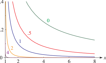
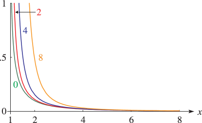
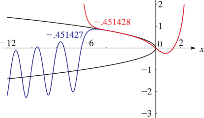
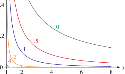
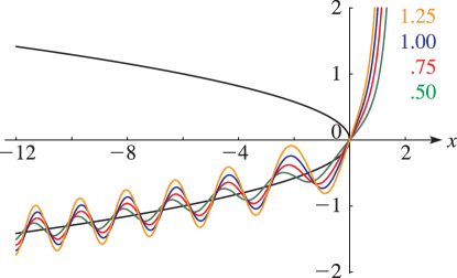
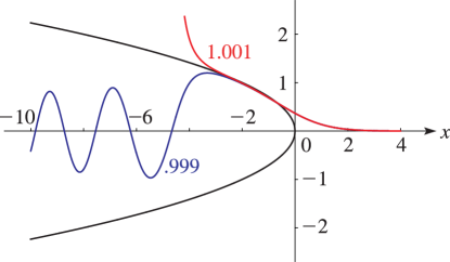
Figure 32.3.1: $w_k(x)$ for $-12\le x\le 1.33$ and $k=0.5$, $0.75$, $1$, $1.25$, and the parabola $6w^2+x=0$, shown in black. Magnify

►

►►

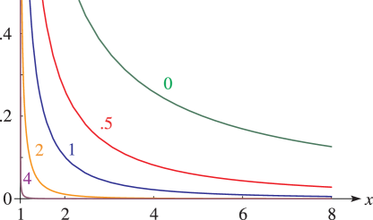
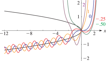
Figure 32.3.2: $w_k(x)$ for $-12\le x\le 2.43$ and $k=-0.5$, $-0.25$, $0$, $1$, $2$, and the parabola $6w^2+x=0$, shown in black. Magnify

►

►►

Figure 32.3.3: $w_k(x)$ for $-12\le x\le 0.73$ and $k=\mathrm{1.85185\hspace{0.33em}3}$, $\mathrm{1.85185\hspace{0.33em}5}$. …The parabola $6w^2+x=0$ is shown in black. Magnify

►

►►

Figure 32.3.4: $w_k(x)$ for $-12\le x\le 2.3$ and $k=-\mathrm{0.45142\hspace{0.33em}7}$, $-\mathrm{0.45142\hspace{0.33em}8}$. …The parabola $6w^2+x=0$ is shown in black. Magnify

… ►

►►

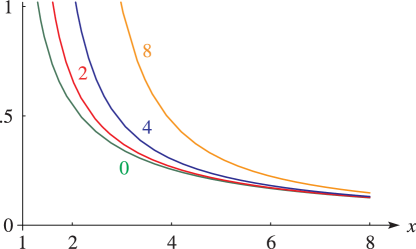
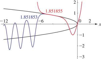
Figure 32.3.6: $w_k(x)$ for $-10\le x\le 4$ with $k=0.999$, $1.001$. …The parabola $2w^2+x=0$ is shown in black. Magnify

…

6: 14.12 Integral Representations

… ►

14.12.9 $${𝑸}_n^m\left(x\right)=\frac{1}{n!}{\int }_0^u{\left(x-{\left(x^2-1\right)}^{1/2}\cosh t\right)}^n\cosh \left(mt\right)dt,$$

ⓘ

Symbols:

${𝑸}_{\nu }^{\mu }\left(z\right)$: Olver’s associated Legendre function, $dx$: differential of $x$ , $!$: factorial (as in $n!$), $\cosh z$: hyperbolic cosine function, $\int$: integral, $x$: real variable, $m$: nonnegative integer, $n$: nonnegative integer and $u$

Permalink:

http://dlmf.nist.gov/14.12.E9

Encodings:

pMML, png, TeX

See also:

Annotations for §14.12(ii), §14.12 and Ch.14

… ►

14.12.11 $${𝑸}_n^m\left(x\right)=\frac{{\left(x^2-1\right)}^{m/2}}{2^{n+1}n!}{\int }_{-1}^1\frac{{\left(1-t^2\right)}^n}{{(x-t)}^{n+m+1}}dt,$$

ⓘ

Symbols:

${𝑸}_{\nu }^{\mu }\left(z\right)$: Olver’s associated Legendre function, $dx$: differential of $x$ , $!$: factorial (as in $n!$), $\int$: integral, $x$: real variable, $m$: nonnegative integer and $n$: nonnegative integer

Permalink:

http://dlmf.nist.gov/14.12.E11

Encodings:

pMML, png, TeX

See also:

Annotations for §14.12(ii), §14.12 and Ch.14

►

14.12.12 $${𝑸}_n^m\left(x\right)=\frac{1}{(n-m)!}{P}_n^m\left(x\right){\int }_x^{\mathrm{\infty }}\frac{dt}{\left(t^2-1\right){\left(P_n^m\left(t\right)\right)}^2},$$ $n\ge m$.

ⓘ

Symbols:

$P_{\nu }^{\mu }\left(z\right)$: associated Legendre function of the first kind, ${𝑸}_{\nu }^{\mu }\left(z\right)$: Olver’s associated Legendre function, $dx$: differential of $x$ , $!$: factorial (as in $n!$), $\int$: integral, $x$: real variable, $m$: nonnegative integer and $n$: nonnegative integer

Referenced by:

§14.17(i)

Permalink:

http://dlmf.nist.gov/14.12.E12

Encodings:

pMML, png, TeX

See also:

Annotations for §14.12(ii), §14.12 and Ch.14

… ►

14.12.13 $${𝑸}_n\left(x\right)=\frac{1}{2(n!)}{\int }_{-1}^1\frac{P_n\left(t\right)}{x-t}dt.$$

ⓘ

Symbols:

$P_n\left(x\right)$: Legendre polynomial, $dx$: differential of $x$ , $!$: factorial (as in $n!$), $\int$: integral, ${𝑸}_{\nu }\left(z\right)={𝑸}_{\nu }^0\left(z\right)$: Olver’s associated Legendre function, $x$: real variable and $n$: nonnegative integer

A&S Ref:

8.8.3 (modified)

Permalink:

http://dlmf.nist.gov/14.12.E13

Encodings:

pMML, png, TeX

See also:

Annotations for §14.12(ii), §14.12(ii), §14.12 and Ch.14

… ►

14.12.14 $${𝑸}_n\left(x\right)=\frac{1}{n!}{\int }_0^{\mathrm{\infty }}\frac{dt}{{\left(x+{(x^2-1)}^{1/2}\cosh t\right)}^{n+1}}.$$

ⓘ

Symbols:

$dx$: differential of $x$ , $!$: factorial (as in $n!$), $\cosh z$: hyperbolic cosine function, $\int$: integral, ${𝑸}_{\nu }\left(z\right)={𝑸}_{\nu }^0\left(z\right)$: Olver’s associated Legendre function, $x$: real variable and $n$: nonnegative integer

Permalink:

http://dlmf.nist.gov/14.12.E14

Encodings:

pMML, png, TeX

See also:

Annotations for §14.12(ii), §14.12(ii), §14.12 and Ch.14

…

7: 14.9 Connection Formulas

… ►

§14.9(iii) Connections Between $P_{\nu }^{\pm \mu }\left(x\right)$, $P_{-\nu -1}^{\pm \mu }\left(x\right)$, ${𝑸}_{\nu }^{\pm \mu }\left(x\right)$, ${𝑸}_{-\nu -1}^{\mu }\left(x\right)$

… ►

14.9.12 $$\cos \left(\nu \pi \right)P_{\nu }^{-\mu }\left(x\right)=-\frac{{𝑸}_{\nu }^{\mu }\left(x\right)}{\mathrm{\Gamma }\left(\mu -\nu \right)}+\frac{{𝑸}_{-\nu -1}^{\mu }\left(x\right)}{\mathrm{\Gamma }\left(\nu +\mu +1\right)}.$$

ⓘ

Symbols:

$\mathrm{\Gamma }\left(z\right)$: gamma function, $P_{\nu }^{\mu }\left(z\right)$: associated Legendre function of the first kind, ${𝑸}_{\nu }^{\mu }\left(z\right)$: Olver’s associated Legendre function, $\pi$: the ratio of the circumference of a circle to its diameter, $\cos z$: cosine function, $x$: real variable, $\mu$: general order and $\nu$: general degree

A&S Ref:

8.2.2 (modified)

Referenced by:

§14.20(i), §14.8(ii), §14.8(iii)

Permalink:

http://dlmf.nist.gov/14.9.E12

Encodings:

pMML, png, TeX

See also:

Annotations for §14.9(iii), §14.9 and Ch.14

… ►

14.9.14 $${𝑸}_{\nu }^{-\mu }\left(x\right)={𝑸}_{\nu }^{\mu }\left(x\right),$$

ⓘ

Symbols:

${𝑸}_{\nu }^{\mu }\left(z\right)$: Olver’s associated Legendre function, $x$: real variable, $\mu$: general order and $\nu$: general degree

A&S Ref:

8.2.6 (modified)

Referenced by:

§14.23, §14.9(iv)

Permalink:

http://dlmf.nist.gov/14.9.E14

Encodings:

pMML, png, TeX

See also:

Annotations for §14.9(iii), §14.9 and Ch.14

… ►

14.9.16 $${𝑸}_{\nu }^{\mu }\left(x\right)={\left(\frac{1}{2}\pi \right)}^{1/2}{\left(x^2-1\right)}^{-1/4}{P}_{-\mu -(1/2)}^{-\nu -(1/2)}\left(x{\left(x^2-1\right)}^{-1/2}\right).$$

ⓘ

Symbols:

$P_{\nu }^{\mu }\left(z\right)$: associated Legendre function of the first kind, ${𝑸}_{\nu }^{\mu }\left(z\right)$: Olver’s associated Legendre function, $\pi$: the ratio of the circumference of a circle to its diameter, $x$: real variable, $\mu$: general order and $\nu$: general degree

A&S Ref:

8.2.7 (modified)

Referenced by:

§14.19(v), §14.21(iii), §14.9(iv)

Permalink:

http://dlmf.nist.gov/14.9.E16

Encodings:

pMML, png, TeX

See also:

Annotations for §14.9(iv), §14.9 and Ch.14

… ►

14.9.17 $$P_{\nu }^{\mu }\left(x\right)={(2/\pi )}^{1/2}{\left(x^2-1\right)}^{-1/4}{𝑸}_{-\mu -(1/2)}^{\nu +(1/2)}\left(x{\left(x^2-1\right)}^{-1/2}\right).$$

ⓘ

Symbols:

$P_{\nu }^{\mu }\left(z\right)$: associated Legendre function of the first kind, ${𝑸}_{\nu }^{\mu }\left(z\right)$: Olver’s associated Legendre function, $\pi$: the ratio of the circumference of a circle to its diameter, $x$: real variable, $\mu$: general order and $\nu$: general degree

Referenced by:

§14.19(v), §14.9(iv)

Permalink:

http://dlmf.nist.gov/14.9.E17

Encodings:

pMML, png, TeX

See also:

Annotations for §14.9(iv), §14.9 and Ch.14

8: 14.22 Graphics

… ►

►

►

Figure 14.22.4: ${𝑸}_0^0\left(x+\mathrm{i}y\right)$, $-5\le x\le 5$, $-5\le y\le 5$. … Magnify 3D Help

9: 14.19 Toroidal (or Ring) Functions

… ►Most required properties of toroidal functions come directly from the results for $P_{\nu }^{\mu }\left(x\right)$ and ${𝑸}_{\nu }^{\mu }\left(x\right)$. … ►

14.19.5 $${𝑸}_{n-\frac{1}{2}}^m\left(\cosh \xi \right)=\frac{\mathrm{\Gamma }\left(n+\frac{1}{2}\right)}{\mathrm{\Gamma }\left(n+m+\frac{1}{2}\right)\mathrm{\Gamma }\left(n-m+\frac{1}{2}\right)}{\int }_0^{\mathrm{\infty }}\frac{\cosh \left(mt\right)}{{(\cosh \xi +\cosh t\sinh \xi )}^{n+(1/2)}}dt,$$ .

ⓘ

Symbols:

$\mathrm{\Gamma }\left(z\right)$: gamma function, ${𝑸}_{\nu }^{\mu }\left(z\right)$: Olver’s associated Legendre function, $dx$: differential of $x$ , $\cosh z$: hyperbolic cosine function, $\sinh z$: hyperbolic sine function, $\int$: integral, $m$: nonnegative integer, $n$: nonnegative integer and $\xi >0$: variable

A&S Ref:

8.11.4 (modified and corrected)

Permalink:

http://dlmf.nist.gov/14.19.E5

Encodings:

pMML, png, TeX

See also:

Annotations for §14.19(iii), §14.19 and Ch.14

… ►

14.19.6 $${𝑸}_{-\frac{1}{2}}^{\mu }\left(\cosh \xi \right)+2\sum _{n=1}^{\mathrm{\infty }}\frac{\mathrm{\Gamma }\left(\mu +n+\frac{1}{2}\right)}{\mathrm{\Gamma }\left(\mu +\frac{1}{2}\right)}{𝑸}_{n-\frac{1}{2}}^{\mu }\left(\cosh \xi \right)\cos \left(n\varphi \right)=\frac{{\left(\frac{1}{2}\pi \right)}^{1/2}{\left(\sinh \xi \right)}^{\mu }}{{\left(\cosh \xi -\cos \varphi \right)}^{\mu +(1/2)}},$$ $\mathrm{\Re }\mu >-\frac{1}{2}$.

ⓘ

Symbols:

$\mathrm{\Gamma }\left(z\right)$: gamma function, ${𝑸}_{\nu }^{\mu }\left(z\right)$: Olver’s associated Legendre function, $\pi$: the ratio of the circumference of a circle to its diameter, $\cos z$: cosine function, $\cosh z$: hyperbolic cosine function, $\sinh z$: hyperbolic sine function, $\mathrm{\Re }$: real part, $n$: nonnegative integer, $\mu$: general order and $\xi >0$: variable

Permalink:

http://dlmf.nist.gov/14.19.E6

Encodings:

pMML, png, TeX

See also:

Annotations for §14.19(iv), §14.19 and Ch.14

… ►

14.19.7 $$P_{n-\frac{1}{2}}^m\left(\cosh \xi \right)=\frac{\mathrm{\Gamma }\left(n+m+\frac{1}{2}\right)}{\mathrm{\Gamma }\left(n-m+\frac{1}{2}\right)}{\left(\frac{2}{\pi \sinh \xi }\right)}^{1/2}{𝑸}_{m-\frac{1}{2}}^n\left(\coth \xi \right),$$

ⓘ

Symbols:

$\mathrm{\Gamma }\left(z\right)$: gamma function, $P_{\nu }^{\mu }\left(z\right)$: associated Legendre function of the first kind, ${𝑸}_{\nu }^{\mu }\left(z\right)$: Olver’s associated Legendre function, $\pi$: the ratio of the circumference of a circle to its diameter, $\cosh z$: hyperbolic cosine function, $\coth z$: hyperbolic cotangent function, $\sinh z$: hyperbolic sine function, $m$: nonnegative integer, $n$: nonnegative integer and $\xi >0$: variable

Permalink:

http://dlmf.nist.gov/14.19.E7

Encodings:

pMML, png, TeX

See also:

Annotations for §14.19(v), §14.19 and Ch.14

►

14.19.8 $${𝑸}_{n-\frac{1}{2}}^m\left(\cosh \xi \right)=\frac{\mathrm{\Gamma }\left(m-n+\frac{1}{2}\right)}{\mathrm{\Gamma }\left(m+n+\frac{1}{2}\right)}{\left(\frac{\pi }{2\sinh \xi }\right)}^{1/2}{P}_{m-\frac{1}{2}}^n\left(\coth \xi \right).$$

ⓘ

Symbols:

$\mathrm{\Gamma }\left(z\right)$: gamma function, $P_{\nu }^{\mu }\left(z\right)$: associated Legendre function of the first kind, ${𝑸}_{\nu }^{\mu }\left(z\right)$: Olver’s associated Legendre function, $\pi$: the ratio of the circumference of a circle to its diameter, $\cosh z$: hyperbolic cosine function, $\coth z$: hyperbolic cotangent function, $\sinh z$: hyperbolic sine function, $m$: nonnegative integer, $n$: nonnegative integer and $\xi >0$: variable

Permalink:

http://dlmf.nist.gov/14.19.E8

Encodings:

pMML, png, TeX

See also:

Annotations for §14.19(v), §14.19 and Ch.14

10: 14.25 Integral Representations

… ►The principal values of $P_{\nu }^{-\mu }\left(z\right)$ and ${𝑸}_{\nu }^{\mu }\left(z\right)$ (§14.21(i)) are given by … ►

14.25.2 $${𝑸}_{\nu }^{\mu }\left(z\right)=\frac{{\pi }^{1/2}{\left(z^2-1\right)}^{\mu /2}}{2^{\mu }\mathrm{\Gamma }\left(\mu +\frac{1}{2}\right)\mathrm{\Gamma }\left(\nu -\mu +1\right)}{\int }_0^{\mathrm{\infty }}\frac{{(\sinh t)}^{2\mu }}{{\left(z+{(z^2-1)}^{1/2}\cosh t\right)}^{\nu +\mu +1}}dt,$$ $\mathrm{\Re }\left(\nu +1\right)>\mathrm{\Re }\mu >-\frac{1}{2}$,

ⓘ

Symbols:

$\mathrm{\Gamma }\left(z\right)$: gamma function, ${𝑸}_{\nu }^{\mu }\left(z\right)$: Olver’s associated Legendre function, $\pi$: the ratio of the circumference of a circle to its diameter, $dx$: differential of $x$ , $\cosh z$: hyperbolic cosine function, $\sinh z$: hyperbolic sine function, $\int$: integral, $\mathrm{\Re }$: real part, $z$: complex variable, $\mu$: general order and $\nu$: general degree

Referenced by:

§14.25

Permalink:

http://dlmf.nist.gov/14.25.E2

Encodings:

pMML, png, TeX

See also:

Annotations for §14.25 and Ch.14

…