difference operators

SearchAdvancedHelp

(0.002 seconds)

11—20 of 40 matching pages

11: 3.10 Continued Fractions

… ►($\nabla$ is the backward difference operator.) …

12: 26.8 Set Partitions: Stirling Numbers

… ►

26.8.31 $$\frac{1}{k!}\frac{d^k}{{dx}^k}f(x)=\sum _{n=k}^{\mathrm{\infty }}\frac{s(n,k)}{n!}{\mathrm{\Delta }}^{n}f(x),$$

ⓘ

Symbols:

$s(n,k)$: Stirling number of the first kind, $\frac{df}{dx}$: derivative of $f$ with respect to $x$ , $!$: factorial (as in $n!$), $\mathrm{\Delta }$: forward difference operator, $x$: real variable, $k$: nonnegative integer and $n$: nonnegative integer

A&S Ref:

24.1.3

Referenced by:

§26.8(v)

Permalink:

http://dlmf.nist.gov/26.8.E31

Encodings:

pMML, png, TeX

See also:

Annotations for §26.8(v), §26.8 and Ch.26

… ►

26.8.32 $$\mathrm{\Delta }f(x)=f(x+1)-f(x);$$

ⓘ

Symbols:

$\mathrm{\Delta }$: forward difference operator and $x$: real variable

Permalink:

http://dlmf.nist.gov/26.8.E32

Encodings:

pMML, png, TeX

See also:

Annotations for §26.8(v), §26.8 and Ch.26

… ►

26.8.37 $$\frac{1}{k!}{\mathrm{\Delta }}^{k}f(x)=\sum _{n=k}^{\mathrm{\infty }}\frac{S(n,k)}{n!}\frac{d^n}{{dx}^n}f(x),$$

ⓘ

Symbols:

$S(n,k)$: Stirling number of the second kind, $\frac{df}{dx}$: derivative of $f$ with respect to $x$ , $!$: factorial (as in $n!$), $\mathrm{\Delta }$: forward difference operator, $x$: real variable, $k$: nonnegative integer and $n$: nonnegative integer

A&S Ref:

24.1.4

Referenced by:

§26.8(v)

Permalink:

http://dlmf.nist.gov/26.8.E37

Encodings:

pMML, png, TeX

See also:

Annotations for §26.8(v), §26.8 and Ch.26

…

13: 18.19 Hahn Class: Definitions

… ►The Askey scheme extends the three families of classical OP’s (Jacobi, Laguerre and Hermite) with eight further families of OP’s for which the role of the differentiation operator $\frac{d}{dx}$ in the case of the classical OP’s is played by a suitable difference operator. … ►

Hahn class (or linear lattice class). These are OP’s $p_n(x)$ where the role of $\frac{d}{dx}$ is played by ${\mathrm{\Delta }}_x$ or ${\nabla }_x$ or ${\delta }_x$ (see §18.1(i) for the definition of these operators). The Hahn class consists of four discrete and two continuous families.

►

Wilson class (or quadratic lattice class). These are OP’s $p_n(x)=p_n(\lambda (y))$ ($p_n(x)$ of degree $n$ in $x$, $\lambda (y)$ quadratic in $y$) where the role of the differentiation operator is played by $\frac{{\mathrm{\Delta }}_y}{{\mathrm{\Delta }}_y(\lambda (y))}$ or $\frac{{\nabla }_y}{{\nabla }_y(\lambda (y))}$ or $\frac{{\delta }_y}{{\delta }_y(\lambda (y))}$. The Wilson class consists of two discrete and two continuous families.

…

14: Bibliography D

… ►

Differential-difference operators associated to reflection groups. Trans. Amer. Math. Soc. 311 (1), pp. 167–183.

ⓘ

External Links:

ISSN 0002-9947, Link, MathReview (W. A. Al-Salam), ZentralBlatt

Referenced by:

§18.38(iii).

Encodings:

BibTeX

…

15: 18.27 $q$-Hahn Class

… ►The $q$-Hahn class OP’s comprise systems of OP’s $\{p_n(x)\}$, $n=0,1,\mathrm{\dots },N$, or $n=0,1,2,\mathrm{\dots }$, that are eigenfunctions of a second order $q$-difference operator. …

16: 18.28 Askey–Wilson Class

… ► $y$) such that $P_n(z)=p_n(\frac{1}{2}(z+z^{-1}))$ in the Askey–Wilson case, and $P_n(y)=p_n(q^{-y}+c{q}^{y+1})$ in the $q$-Racah case, and both are eigenfunctions of a second order $q$-difference operator similar to (18.27.1). …

17: 3.3 Interpolation

… ►

§3.3(iii) Divided Differences

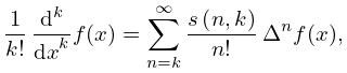
… ►Explicitly, the divided difference of order $n$ is given by … ►This represents the Lagrange interpolation polynomial in terms of divided differences: …Newton’s formula has the advantage of allowing easy updating: incorporation of a new point $z_{n+1}$ requires only addition of the term with $\left[z_0,z_1,\mathrm{\dots },z_{n+1}\right]f$ to (3.3.38), plus the computation of this divided difference. …For example, for $k+1$ coincident points the limiting form is given by $\left[z_0,z_0,\mathrm{\dots },z_0\right]f=f^{(k)}(z_0)/k!$. …

18: 18.38 Mathematical Applications

… ►The Dunkl type operator is a $q$-difference-reflection operator acting on Laurent polynomials and its eigenfunctions, the nonsymmetric Askey–Wilson polynomials, are linear combinations of the symmetric Laurent polynomial $R_n(z;a,b,c,d|q)$ and the ‘anti-symmetric’ Laurent polynomial $z^{-1}(1-az)(1-bz)R_{n-1}(z;qa,qb,c,d|q)$, where $R_n(z)$ is given in (18.28.1_5). …

19: 10.21 Zeros

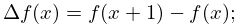
… ►For sign properties of the forward differences that are defined by ►

$$\mathrm{\Delta }{\rho }_{\nu }(t)={\rho }_{\nu }(t+1)-{\rho }_{\nu }(t),$$

►

$${\mathrm{\Delta }}^2{\rho }_{\nu }(t)=\mathrm{\Delta }{\rho }_{\nu }(t+1)-\mathrm{\Delta }{\rho }_{\nu }(t),\mathrm{\dots },$$

… ► … ►Higher coefficients in the asymptotic expansions in this subsection can be obtained by expressing the cross-products in terms of the modulus and phase functions (§10.18), and then reverting the asymptotic expansion for the difference of the phase functions. …

20: Errata

… ►

In the online version, the leading divided difference operators were previously omitted from these formulas, due to programming error.

Reported by Nico Temme on 2021-06-01

…