derivatives with respect to order

SearchAdvancedHelp

(0.010 seconds)

31—40 of 93 matching pages

31: 10.45 Functions of Imaginary Order

§10.45 Functions of Imaginary Order

… ►and ${\tilde{I}}_{\nu }\left(x\right)$, ${\tilde{K}}_{\nu }\left(x\right)$ are real and linearly independent solutions of (10.45.1): … ►The corresponding result for ${\tilde{K}}_{\nu }\left(x\right)$ is given by … ► … ►

32: 2.6 Distributional Methods

… ►

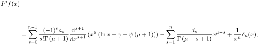
2.6.46 $${𝐼}^{\mu }f(x)=\sum _{s=0}^{n-1}\frac{{(-1)}^s{a}_s}{s!\mathrm{\Gamma }\left(\mu +1\right)}\frac{d^{s+1}}{{dx}^{s+1}}\left(x^{\mu }\left(\ln x-\gamma -\psi \left(\mu +1\right)\right)\right)-\sum _{s=1}^n\frac{d_s}{\mathrm{\Gamma }\left(\mu -s+1\right)}{x}^{\mu -s}+\frac{1}{x^n}{\delta }_n(x),$$

ⓘ

Symbols:

$\mathrm{\Gamma }\left(z\right)$: gamma function, $\gamma$: Euler’s constant, $\frac{df}{dx}$: derivative of $f$ with respect to $x$ , $\psi \left(z\right)$: psi (or digamma) function, $!$: factorial (as in $n!$), $\ln z$: principal branch of logarithm function, $d_s$: coefficients, $\mu$: order, ${𝐼}^{\mu }$: fractional integral , $f(t)$: locally integrable function, $n$: nonnegative integer, $a_n$: coefficients and ${\delta }_n(x)$: sum

Permalink:

http://dlmf.nist.gov/2.6.E46

Encodings:

pMML, png, TeX

See also:

Annotations for §2.6(iii), §2.6 and Ch.2

…

33: 10.1 Special Notation

… ►For the spherical Bessel functions and modified spherical Bessel functions the order $n$ is a nonnegative integer. For the other functions when the order $\nu$ is replaced by $n$, it can be any integer. For the Kelvin functions the order $\nu$ is always assumed to be real. … ►Abramowitz and Stegun (1964): $j_n(z)$, $y_n(z)$, $h_n^{(1)}(z)$, $h_n^{(2)}(z)$, for ${𝗃}_n\left(z\right)$, ${𝗒}_n\left(z\right)$, ${𝗁}_n^{(1)}\left(z\right)$, ${𝗁}_n^{(2)}\left(z\right)$, respectively, when $n\ge 0$. … ►For older notations see British Association for the Advancement of Science (1937, pp. xix–xx) and Watson (1944, Chapters 1–3).

34: 1.5 Calculus of Two or More Variables

… ►

§1.5(i) Partial Derivatives

… ►

Chain Rule

… ►where $f$ and its partial derivatives on the right-hand side are evaluated at $(a,b)$, and $R_n/{({\lambda }^2+{\mu }^2)}^{n/2}\to 0$ as $(\lambda ,\mu )\to (0,0)$. … ►

Change of Order of Integration

… ►

§1.5(vi) Jacobians and Change of Variables

…

35: 14.6 Integer Order

§14.6 Integer Order

►

§14.6(i) Nonnegative Integer Orders

… ►

§14.6(ii) Negative Integer Orders

… ►For connections between positive and negative integer orders see (14.9.3), (14.9.4), and (14.9.13). …

36: 3.7 Ordinary Differential Equations

… ►Consideration will be limited to ordinary linear second-order differential equations … ►

First-Order Equations

… ►The order estimate $O\left(h^5\right)$ holds if the solution $w(z)$ has five continuous derivatives. ►

Second-Order Equations

… ►The order estimates $O\left(h^5\right)$ hold if the solution $w(z)$ has five continuous derivatives. …

37: 1.18 Linear Second Order Differential Operators and Eigenfunction Expansions

§1.18 Linear Second Order Differential Operators and Eigenfunction Expansions

… ►For $T$ to be actually self adjoint it is necessary to also show that $𝒟(T^{\ast })=𝒟(T)$, as it is often the case that $T$ and $T^{\ast }$ have different domains, see Friedman (1990, p 148) for a simple example of such differences involving the differential operator $\frac{d}{dx}$. … ►

§1.18(iv) Formally Self-adjoint Linear Second Order Differential Operators

… ►The special form of (1.18.28) is especially useful for applications in physics, as the connection to non-relativistic quantum mechanics is immediate: $-\frac{d^2}{{dx}^2}$ being proportional to the kinetic energy operator for a single particle in one dimension, $q(x)$ being proportional to the potential energy, often written as $V(x)$, of that same particle, and which is simply a multiplicative operator. … ►The materials developed here follow from the extensions of the Sturm–Liouville theory of second order ODEs as developed by Weyl, to include the limit point and limit circle singular cases. …

38: 31.14 General Fuchsian Equation

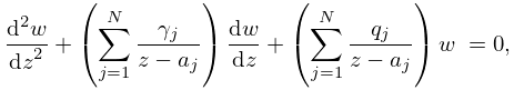
… ►The general second-order Fuchsian equation with $N+1$ regular singularities at $z=a_j$, $j=1,2,\mathrm{\dots },N$, and at $\mathrm{\infty }$, is given by ►

31.14.1 $$\frac{d^{2}w}{{dz}^2}+\left(\sum _{j=1}^N\frac{{\gamma }_j}{z-a_j}\right)\frac{dw}{dz}+\left(\sum _{j=1}^N\frac{q_j}{z-a_j}\right)w=0,$$ ${\sum }_{j=1}^N{q}_j=0$.

ⓘ

Symbols:

$\frac{df}{dx}$: derivative of $f$ with respect to $x$ , $z$: complex variable, $\gamma$: real or complex parameter, $j$: nonnegative integer, $a$: complex parameter, $q$: real or complex parameter and $N+1$: number of singularities

Referenced by:

§31.15(i)

Permalink:

http://dlmf.nist.gov/31.14.E1

Encodings:

pMML, png, TeX

See also:

Annotations for §31.14(i), §31.14 and Ch.31

… ►Heun’s equation (31.2.1) corresponds to $N=3$. ►

Normal Form

… ►An algorithm given in Kovacic (1986) determines if a given (not necessarily Fuchsian) second-order homogeneous linear differential equation with rational coefficients has solutions expressible in finite terms (Liouvillean solutions). …

39: 32.2 Differential Equations

… ►The six equations are sometimes referred to as the Painlevé transcendents, but in this chapter this term will be used only for their solutions. … ►be a nonlinear second-order differential equation in which $F$ is a rational function of $w$ and $dw/dz$, and is locally analytic in $z$, that is, analytic except for isolated singularities in $ℂ$. …An equation is said to have the Painlevé property if all its solutions are free from movable branch points; the solutions may have movable poles or movable isolated essential singularities (§1.10(iii)), however. … ►The fifty equations can be reduced to linear equations, solved in terms of elliptic functions (Chapters 22 and 23), or reduced to one of ${\text{P}}_{\text{I}}$–${\text{P}}_{\text{VI}}$. … ►thus in the limit as $ϵ\to 0$, $W(\zeta )$ satisfies ${\text{P}}_{\text{I}}$ with $z=\zeta$. …

40: 2.8 Differential Equations with a Parameter

… ►dots denoting differentiations with respect to $\xi$. Then … ►The expansions (2.8.11) and (2.8.12) are both uniform and differentiable with respect to $\xi$. … ►The expansions (2.8.15) and (2.8.16) are both uniform and differentiable with respect to $\xi$. … ►The expansions (2.8.25) and (2.8.26) are both uniform and differentiable with respect to $\xi$. …