About the Project

complex

AdvancedHelp

(0.000 seconds)

1—10 of 636 matching pages

1: 31.3 Basic Solutions
31.3.2 a γ c 1 q c 0 = 0 ,
31.3.7 ( 1 z ) 1 δ H ( 1 a , ( ( 1 a ) γ + ϵ ) ( 1 δ ) + α β q ; α + 1 δ , β + 1 δ , 2 δ , γ ; 1 z ) .
2: 37.6 Plane with Weight Function e x 2 y 2
§37.6(i) Complex Circular Hermite Polynomials
As a special case of (37.2.20) define for m , n 0 the (complex) circular Hermite polynomials (first introduced by Itô (1952, §12)) by …Then the polynomials S m , n m ( x + i y , x i y ) ( m = 0 , 1 , , n ) form an orthogonal basis of the space 𝒱 n of complex-valued orthogonal polynomials of degree n on 2 with weight function e x 2 y 2 . … The definition of S m , n ( z , z ¯ ) can be extended to S m , n ( z 1 , z 2 ) , where z 1 and z 2 are two independent complex variables. … and, for the orthogonal basis (37.6.3) of complex circular Hermite polynomials, …
3: 20.12 Mathematical Applications
§20.12(ii) Uniformization and Embedding of Complex Tori
For the terminology and notation see McKean and Moll (1999, pp. 48–53). The space of complex tori / ( + τ ) (that is, the set of complex numbers z in which two of these numbers z 1 and z 2 are regarded as equivalent if there exist integers m , n such that z 1 z 2 = m + τ n ) is mapped into the projective space P 3 via the identification z ( θ 1 ( 2 z | τ ) , θ 2 ( 2 z | τ ) , θ 3 ( 2 z | τ ) , θ 4 ( 2 z | τ ) ) . Thus theta functions “uniformize” the complex torus. This ability to uniformize multiply-connected spaces (manifolds), or multi-sheeted functions of a complex variable (Riemann (1899), Rauch and Lebowitz (1973), Siegel (1988)) has led to applications in string theory (Green et al. (1988a, b), Krichever and Novikov (1989)), and also in statistical mechanics (Baxter (1982)). …
4: 31.1 Special Notation
x , y real variables.
z , ζ , w , W complex variables.
a complex parameter, | a | 1 , a 1 .
q , α , β , γ , δ , ϵ , ν complex parameters.
5: 15.7 Continued Fractions
15.7.1 𝐅 ( a , b ; c ; z ) 𝐅 ( a , b + 1 ; c + 1 ; z ) = t 0 u 1 z t 1 u 2 z t 2 u 3 z t 3 ,
6: 4.34 Derivatives and Differential Equations
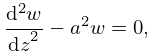
4.34.7 d 2 w d z 2 a 2 w = 0 ,
4.34.8 ( d w d z ) 2 a 2 w 2 = 1 ,
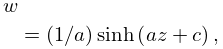
4.34.12 w = ( 1 / a ) sinh ( a z + c ) ,
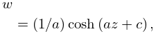
4.34.13 w = ( 1 / a ) cosh ( a z + c ) ,
4.34.14 w = ( 1 / a ) coth ( a z + c ) ,
7: 15.5 Derivatives and Contiguous Functions
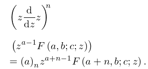
15.5.5 ( z d d z z ) n ( z c a 1 ( 1 z ) a + b c F ( a , b ; c ; z ) ) = ( c a ) n z c a + n 1 ( 1 z ) a n + b c F ( a n , b ; c ; z ) .
8: 32.12 Asymptotic Approximations for Complex Variables
§32.12 Asymptotic Approximations for Complex Variables
9: 4.20 Derivatives and Differential Equations
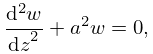
4.20.9 d 2 w d z 2 + a 2 w = 0 ,
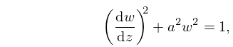
4.20.10 ( d w d z ) 2 + a 2 w 2 = 1 ,
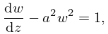
4.20.11 d w d z a 2 w 2 = 1 ,
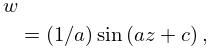
4.20.13 w = ( 1 / a ) sin ( a z + c ) ,
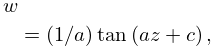
4.20.14 w = ( 1 / a ) tan ( a z + c ) ,
10: 31.12 Confluent Forms of Heun’s Equation
31.12.1 d 2 w d z 2 + ( γ z + δ z 1 + ϵ ) d w d z + α z q z ( z 1 ) w = 0 .
31.12.2 d 2 w d z 2 + ( δ z 2 + γ z + 1 ) d w d z + α z q z 2 w = 0 .
31.12.3 d 2 w d z 2 ( γ z + δ + z ) d w d z + α z q z w = 0 .
31.12.4 d 2 w d z 2 + ( γ + z ) z d w d z + ( α z q ) w = 0 .