…
►Spenceley and Spenceley (1947) tabulates , , , , for and to 12D, or 12 decimals of a radian in the case of .
►Curtis (1964b) tabulates , , for , , and (not ) to 20D.
…
►Zhang and Jin (1996, p. 678) tabulates , , for and to 7D.
…
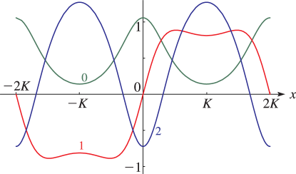
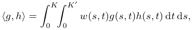
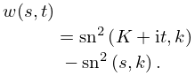
►Figure 22.4.1 illustrates the locations in the -plane of the poles and zeros of the three principal Jacobian functions in the rectangle with vertices , , , .
…
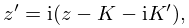
►This half-period will be plus or minus a member of the triple ; the other two members of this triple are quarter periods of .
…
►
Table 22.4.3: Half- or quarter-period shifts of variable for the Jacobian elliptic functions.
►
…
►They are algebraic functions of , , and , and have primitive period .
…
►Lamé–Wangerin functions are solutions of (29.2.1) with the property that is bounded on the line segment from to .
…
…
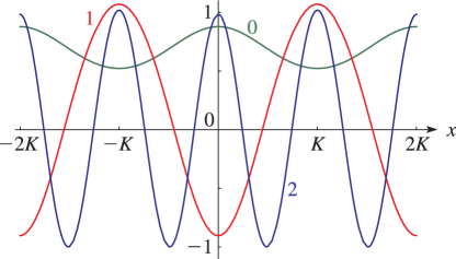
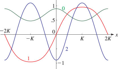
►►►Figure 19.3.1:
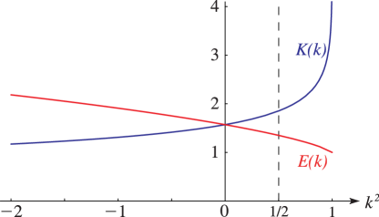
and as functions of for .
Graphs of and are the mirror images in the vertical line .
Magnify
…
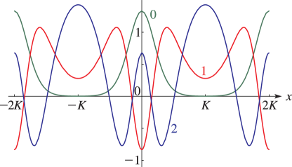
►►
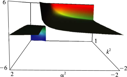
►Figure 19.3.5:
as a function of and for , .
…As it has the limit .
If , then it reduces to .
…
Magnify3DHelp
…
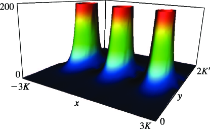
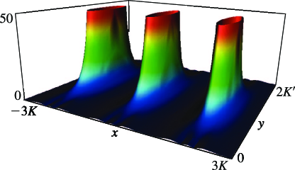
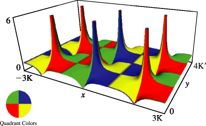
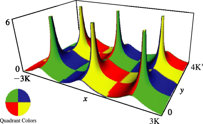
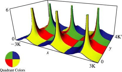
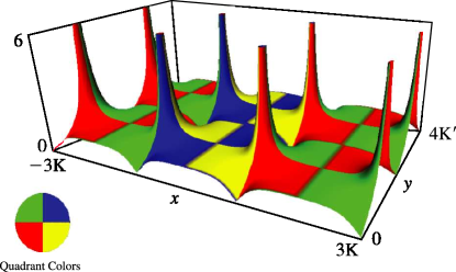
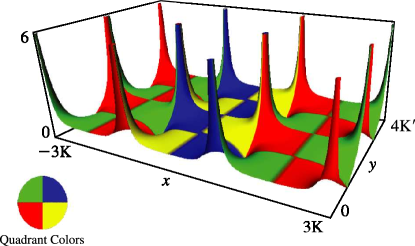
►►
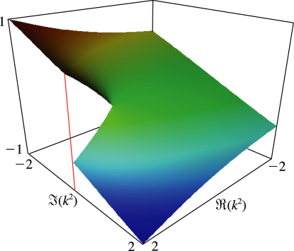
►Figure 19.3.12:
as a function of complex for , .
…On the upper edge of the branch cut () it has the (negative) value , with limit 0 as .
Magnify3DHelp
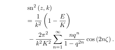
 ►
►
 ►
►
 ►
►
 ►
►
 ►
►
 ►
►
 ►
►
 ►
►
 ►
►
 ►
►
 ►
►
 ►
►
 ►
►
 ►
►
 ►
►
 ►
►
 ►
►
 ►
►
