closed definition

SearchAdvancedHelp

(0.001 seconds)

11—20 of 48 matching pages

11: 9.8 Modulus and Phase

… ►(These definitions of $\theta \left(x\right)$ and $\varphi \left(x\right)$ differ from Abramowitz and Stegun (1964, Chapter 10), and agree more closely with those used in Miller (1946) and Olver (1997b, Chapter 11).) …

12: 3.11 Approximation Techniques

… ►Let $f(x)$ be continuous on a closed interval $[a,b]$. … ►If $f$ is continuously differentiable on $[-1,1]$, then with … ►For general intervals $[a,b]$ we rescale: … ►Let $f$ be continuous on a closed interval $[a,b]$ and $w$ be a continuous nonvanishing function on $[a,b]$: $w$ is called a weight function. …of type $[k,\mathrm{\ell }]$ to $f$ on $[a,b]$ minimizes the maximum value of $\left|{ϵ}_{k,\mathrm{\ell }}(x)\right|$ on $[a,b]$, where …

13: 1.8 Fourier Series

… ►

§1.8(i) Definitions and Elementary Properties

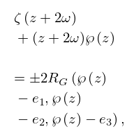
… ►where $f(x)$ is square-integrable on $[-\pi ,\pi ]$ and $a_n,b_n,c_n$ are given by (1.8.2), (1.8.4). … ►For $f(x)$ piecewise continuous on $[a,b]$ and real $\lambda$, … ►If $a_n$ and $b_n$ are the Fourier coefficients of a piecewise continuous function $f(x)$ on $[0,2\pi ]$, then … ►Suppose that $f(x)$ is continuous and of bounded variation on $[0,\mathrm{\infty })$. …

14: 19.25 Relations to Other Functions

… ►

19.25.36 $$\mathrm{\wp }\left(z\right)-e_j\in ℂ\setminus (-\mathrm{\infty },0],$$ $j=1,2,3.$

ⓘ

Symbols:

$\mathrm{\wp }\left(z\right)$ (= $\mathrm{\wp }\left(z|𝕃\right)$ = $\mathrm{\wp }(z;g_2,g_3)$): Weierstrass $\mathrm{\wp }$-function, $e_j$: Weierstrass lattice roots, $ℂ$: complex plane, $\in$: element of, $(a,b]$: half-closed interval, $\setminus$: set subtraction, $j$: $(=1,2,3)$ and $z$: complex number

Referenced by:

(19.25.39)

Permalink:

http://dlmf.nist.gov/19.25.E36

Encodings:

pMML, png, TeX

See also:

Annotations for §19.25(vi), §19.25 and Ch.19

… ►

19.25.37 $$\zeta \left(z+2\omega \right)+(z+2\omega )\mathrm{\wp }\left(z\right)=\pm 2R_G(\mathrm{\wp }\left(z\right)-e_1,\mathrm{\wp }\left(z\right)-e_2,\mathrm{\wp }\left(z\right)-e_3),$$

ⓘ

Symbols:

$R_G(x,y,z)$: symmetric elliptic integral of second kind, $\mathrm{\wp }\left(z\right)$ (= $\mathrm{\wp }\left(z|𝕃\right)$ = $\mathrm{\wp }(z;g_2,g_3)$): Weierstrass $\mathrm{\wp }$-function, $e_j$: Weierstrass lattice roots, $\zeta \left(z\right)$ (= $\zeta \left(z|𝕃\right)$ = $\zeta (z;g_2,g_3)$): Weierstrass zeta function and $z$: complex number

Referenced by:

§19.25(vi), Erratum (V1.0.18) for Equation (19.25.37), Erratum (V1.1.0) for Subsection 19.25(vi)

Permalink:

http://dlmf.nist.gov/19.25.E37

Encodings:

pMML, png, TeX

Correction (effective with 1.1.0):

This equation has been corrected, namely the left-hand side which was originally $\zeta \left(z\right)+z\mathrm{\wp }\left(z\right)$, has been replaced by $\zeta \left(z+2\omega \right)+(z+2\omega )\mathrm{\wp }\left(z\right)$, and the right-hand side has been multiplied by $\pm 1$.

Clarification (effective with 1.0.18):

The Weierstrass zeta function in this equation incorrectly linked to the definition of the Riemann zeta function. However, to the eye, the functions appeared correct.

See also:

Annotations for §19.25(vi), §19.25 and Ch.19

…

15: 4.45 Methods of Computation

… ►The other trigonometric functions can be found from the definitions (4.14.4)–(4.14.7). … ►The hyperbolic functions can be computed directly from the definitions (4.28.1)–(4.28.7). … ►The trigonometric functions may be computed from the definitions (4.14.1)–(4.14.7), and their inverses from the logarithmic forms in §4.23(iv), followed by (4.23.7)–(4.23.9). … ►For $x\in [-1/\mathrm{e},\mathrm{\infty })$ the principal branch $\mathrm{Wp}\left(x\right)$ can be computed by solving the defining equation $W{\mathrm{e}}^W=x$ numerically, for example, by Newton’s rule (§3.8(ii)). … ►Similarly for $\mathrm{Wm}\left(x\right)$ in the interval $[-1/\mathrm{e},0)$. …

16: 4.13 Lambert $W$-Function

§4.13 Lambert $W$-Function

… ►On the $z$-interval $[0,\mathrm{\infty })$ there is one real solution, and it is nonnegative and increasing. … ► $W_0\left(z\right)$ is a single-valued analytic function on $ℂ\setminus (-\mathrm{\infty },-{\mathrm{e}}^{-1}]$, real-valued when $z>-{\mathrm{e}}^{-1}$, and has a square root branch point at $z=-{\mathrm{e}}^{-1}$. …The other branches $W_k\left(z\right)$ are single-valued analytic functions on $ℂ\setminus (-\mathrm{\infty },0]$, have a logarithmic branch point at $z=0$, and, in the case $k=\pm 1$, have a square root branch point at $z=-{\mathrm{e}}^{-1}\mp 0\mathrm{i}$ respectively. … ►For the definition of Stirling cycle numbers of the first kind $\left[\genfrac{}{}{0.0pt}{}{n}{k}\right]$ see (26.13.3). …

17: 10.2 Definitions

§10.2 Definitions

… ►The principal branch corresponds to the principal branches of $J_{\pm \nu }\left(z\right)$ in (10.2.3) and (10.2.4), with a cut in the $z$-plane along the interval $(-\mathrm{\infty },0]$. … ►

Bessel Functions of the Third Kind (Hankel Functions)

… ►The principal branches correspond to principal values of the square roots in (10.2.5) and (10.2.6), again with a cut in the $z$-plane along the interval $(-\mathrm{\infty },0]$. … ►

Cylinder Functions

…

18: 6.2 Definitions and Interrelations

§6.2 Definitions and Interrelations

►

§6.2(i) Exponential and Logarithmic Integrals

… ►As in the case of the logarithm (§4.2(i)) there is a cut along the interval $(-\mathrm{\infty },0]$ and the principal value is two-valued on $(-\mathrm{\infty },0)$. … ►

§6.2(ii) Sine and Cosine Integrals

… ►

§6.2(iii) Auxiliary Functions

…

19: 4.23 Inverse Trigonometric Functions

… ►

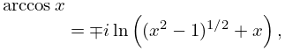
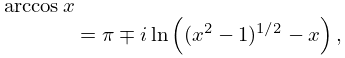
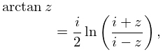
§4.23(i) General Definitions

… ►An equivalent definition is … ►

4.23.24 $$\arccos x=\mp \mathrm{i}\ln \left({(x^2-1)}^{1/2}+x\right),$$ $x\in [1,\mathrm{\infty })$,

ⓘ

Symbols:

$[a,b)$: half-closed interval, $\in$: element of, $\mathrm{i}$: imaginary unit, $\arccos z$: arccosine function, $\ln z$: principal branch of logarithm function and $x$: real variable

Permalink:

http://dlmf.nist.gov/4.23.E24

Encodings:

pMML, png, TeX

See also:

Annotations for §4.23(iv), §4.23(iv), §4.23 and Ch.4

►

4.23.25 $$\arccos x=\pi \mp \mathrm{i}\ln \left({(x^2-1)}^{1/2}-x\right),$$ $x\in (-\mathrm{\infty },-1]$,

ⓘ

Symbols:

$\pi$: the ratio of the circumference of a circle to its diameter, $\in$: element of, $\mathrm{i}$: imaginary unit, $\arccos z$: arccosine function, $\ln z$: principal branch of logarithm function, $(a,b]$: half-closed interval and $x$: real variable

Permalink:

http://dlmf.nist.gov/4.23.E25

Encodings:

pMML, png, TeX

See also:

Annotations for §4.23(iv), §4.23(iv), §4.23 and Ch.4

… ►

4.23.26 $$\arctan z=\frac{\mathrm{i}}{2}\ln \left(\frac{\mathrm{i}+z}{\mathrm{i}-z}\right),$$ $z/\mathrm{i}\in ℂ\setminus (-\mathrm{\infty },-1]\cup [1,\mathrm{\infty })$;

ⓘ

Symbols:

$[a,b)$: half-closed interval, $ℂ$: complex plane, $\in$: element of, $\mathrm{i}$: imaginary unit, $\arctan z$: arctangent function, $\ln z$: principal branch of logarithm function, $(a,b]$: half-closed interval, $\setminus$: set subtraction, $\cup$: union and $z$: complex variable

Referenced by:

§4.23(iv)

Permalink:

http://dlmf.nist.gov/4.23.E26

Encodings:

pMML, png, TeX

See also:

Annotations for §4.23(iv), §4.23(iv), §4.23 and Ch.4

…

20: 26.15 Permutations: Matrix Notation

… ►For $(j,k)\in B$, $B\setminus [j,k]$ denotes $B$ after removal of all elements of the form $(j,t)$ or $(t,k)$, $t=1,2,\mathrm{\dots },n$. … ►

26.15.5 $$R(x,B)=xR(x,B\setminus [j,k])+R(x,B\setminus (j,k)).$$

ⓘ

Symbols:

$[a,b]$: closed interval, $(a,b)$: open interval, $\setminus$: set subtraction, $x$: real variable, $j$: nonnegative integer, $k$: nonnegative integer, $B$: subset and $R(x,B)$: rook polynomial

Permalink:

http://dlmf.nist.gov/26.15.E5

Encodings:

pMML, png, TeX

See also:

Annotations for §26.15 and Ch.26

… ►

26.15.8 $$N_0(B)\equiv N(0,B)=\sum _{k=0}^n{(-1)}^k{r}_k(B)(n-k)!.$$

ⓘ

Symbols:

$\equiv$: equals by definition, $!$: factorial (as in $n!$), $k$: nonnegative integer, $n$: nonnegative integer, $B$: subset, $r_j(B)$: number of rook positions and $N(x,B)$: generating function

Permalink:

http://dlmf.nist.gov/26.15.E8

Encodings:

pMML, png, TeX

See also:

Annotations for §26.15 and Ch.26

… ►

26.15.11 $$\sum _{k=0}^n{r}_{n-k}(B){\left(x-k+1\right)}_k=\prod _{j=1}^n(x+b_j-j+1).$$

ⓘ

Symbols:

${\left(a\right)}_n$: Pochhammer’s symbol (or shifted factorial), $x$: real variable, $j$: nonnegative integer, $k$: nonnegative integer, $n$: nonnegative integer, $B$: subset and $r_j(B)$: number of rook positions

Permalink:

http://dlmf.nist.gov/26.15.E11

Encodings:

pMML, png, TeX

Errata (effective with 1.1.2):

The Pochhammer symbol now links to its definition.

See also:

Annotations for §26.15, §26.15 and Ch.26

… ►

26.15.12 $$\sum _{k=0}^n{r}_{n-k}(B){\left(x-k+1\right)}_k=x^n,$$

ⓘ

Symbols:

${\left(a\right)}_n$: Pochhammer’s symbol (or shifted factorial), $x$: real variable, $k$: nonnegative integer, $n$: nonnegative integer, $B$: subset and $r_j(B)$: number of rook positions

Permalink:

http://dlmf.nist.gov/26.15.E12

Encodings:

pMML, png, TeX

Errata (effective with 1.1.2):

The Pochhammer symbol now links to its definition.

See also:

Annotations for §26.15, §26.15 and Ch.26

…