as%20x%E2%86%92%C2%111

SearchAdvancedHelp

(0.002 seconds)

11—20 of 687 matching pages

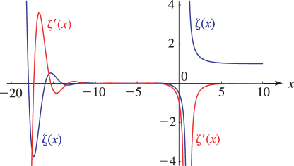
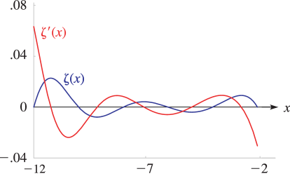
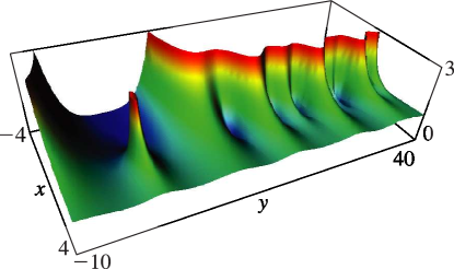
11: 25.3 Graphics

… ►

►►

Figure 25.3.1: Riemann zeta function $\zeta \left(x\right)$ and its derivative ${\zeta }^{\prime }\left(x\right)$, $-20\le x\le 10$. Magnify

►

►►

Figure 25.3.2: Riemann zeta function $\zeta \left(x\right)$ and its derivative ${\zeta }^{\prime }\left(x\right)$, $-12\le x\le -2$. Magnify

►

►

►

Figure 25.3.3: Modulus of the Riemann zeta function $|\zeta \left(x+\mathrm{i}y\right)|$, $-4\le x\le 4$, $-10\le y\le 40$. Magnify 3D Help

…

12: 9.18 Tables

… ►

Miller (1946) tabulates $\mathrm{Ai}\left(x\right)$, ${\mathrm{Ai}}^{\prime }\left(x\right)$ for $x=-20(.01)2;$ ${\log }_{10}\mathrm{Ai}\left(x\right)$, ${\mathrm{Ai}}^{\prime }\left(x\right)/\mathrm{Ai}\left(x\right)$ for $x=0(.1)25(1)75$; $\mathrm{Bi}\left(x\right)$, ${\mathrm{Bi}}^{\prime }\left(x\right)$ for $x=-10(.1)2.5$; ${\log }_{10}\mathrm{Bi}\left(x\right)$, ${\mathrm{Bi}}^{\prime }\left(x\right)/\mathrm{Bi}\left(x\right)$ for $x=0(.1)10$; $M\left(x\right)$, $N\left(x\right)$, $\theta \left(x\right)$, $\varphi \left(x\right)$ (respectively $F(x)$, $G(x)$, $\chi (x)$, $\psi (x)$) for $x=-80(1)-30(.1)0$. Precision is generally 8D; slightly less for some of the auxiliary functions. Extracts from these tables are included in Abramowitz and Stegun (1964, Chapter 10), together with some auxiliary functions for large arguments.

… ►

Zhang and Jin (1996, p. 337) tabulates $\mathrm{Ai}\left(x\right)$, ${\mathrm{Ai}}^{\prime }\left(x\right)$, $\mathrm{Bi}\left(x\right)$, ${\mathrm{Bi}}^{\prime }\left(x\right)$ for $x=0(1)20$ to 8S and for $x=-20(1)0$ to 9D.

… ►

Miller (1946) tabulates $a_k$, ${\mathrm{Ai}}^{\prime }\left(a_k\right)$, $a_k^{\prime }$, $\mathrm{Ai}\left(a_k^{\prime }\right)$, $k=1(1)50$; $b_k$, ${\mathrm{Bi}}^{\prime }\left(b_k\right)$, $b_k^{\prime }$, $\mathrm{Bi}\left(b_k^{\prime }\right)$, $k=1(1)20$. Precision is 8D. Entries for $k=1(1)20$ are reproduced in Abramowitz and Stegun (1964, Chapter 10).

►

Sherry (1959) tabulates $a_k$, ${\mathrm{Ai}}^{\prime }\left(a_k\right)$, $a_k^{\prime }$, $\mathrm{Ai}\left(a_k^{\prime }\right)$, $k=1(1)50$; 20S.

►

Zhang and Jin (1996, p. 339) tabulates $a_k$, ${\mathrm{Ai}}^{\prime }\left(a_k\right)$, $a_k^{\prime }$, $\mathrm{Ai}\left(a_k^{\prime }\right)$, $b_k$, ${\mathrm{Bi}}^{\prime }\left(b_k\right)$, $b_k^{\prime }$, $\mathrm{Bi}\left(b_k^{\prime }\right)$, $k=1(1)20$; 8D.

…

13: 25.12 Polylogarithms

… ►

►►

Figure 25.12.1: Dilogarithm function ${\mathrm{Li}}_2\left(x\right)$, Magnify

►

►

►

Figure 25.12.2: Absolute value of the dilogarithm function $\left|{\mathrm{Li}}_2\left(x+\mathrm{i}y\right)\right|$, $-20\le x\le 20$, $-20\le y\le 20$. … Magnify 3D Help

… ►

$F_s(x)=-{\mathrm{Li}}_{s+1}\left(-{\mathrm{e}}^x\right),$

►

$G_s(x)={\mathrm{Li}}_{s+1}\left({\mathrm{e}}^x\right).$

►For a uniform asymptotic approximation for $F_s(x)$ see Temme and Olde Daalhuis (1990).

14: Bibliography

… ►

Exact linearization of a Painlevé transcendent. Phys. Rev. Lett. 38 (20), pp. 1103–1106.

ⓘ

External Links:

Document, MathReview (Mark Adler)

Referenced by:

§32.11(ii), §32.13(i), §32.13(ii), §32.13(iii), §32.5.

Encodings:

BibTeX

… ►

On the degrees of irreducible factors of higher order Bernoulli polynomials. Acta Arith. 62 (4), pp. 329–342.

ⓘ

External Links:

ISSN 0065-1036, Pdf, MathReview (L. Skula), ZentralBlatt

Referenced by:

§24.12(iii).

Encodings:

BibTeX

… ►

Application of the combined nonlinear-condensation transformation to problems in statistical analysis and theoretical physics. Comput. Phys. Comm. 150 (1), pp. 1–20.

ⓘ

Notes:

Includes algorithms for Lerch’s transcendent. C and Mathematica codes by Aksenov and Jentschura are available.

External Links:

Code, Document

Referenced by:

1st item.

Encodings:

BibTeX

… ►

Repeated integrals and derivatives of $K$ Bessel functions. SIAM J. Math. Anal. 20 (1), pp. 169–175.

ⓘ

External Links:

ISSN 0036-1410, Document, MathReview (A. Haimovici), ZentralBlatt

Referenced by:

§10.43(iii).

Encodings:

BibTeX

… ►

Derivatives and integrals with respect to the order of the Struve functions ${𝐇}_{\nu }(x)$ and ${𝐋}_{\nu }(x)$ . J. Math. Anal. Appl. 137 (1), pp. 17–36.

ⓘ

External Links:

ISSN 0022-247X, Document, MathReview (A. McD. Mercer), ZentralBlatt

Referenced by:

§11.4(vi), §11.7(iv).

Encodings:

BibTeX

…

15: 27.2 Functions

… ►Euclid’s Elements (Euclid (1908, Book IX, Proposition 20)) gives an elegant proof that there are infinitely many primes. …There is great interest in the function $\pi \left(x\right)$ that counts the number of primes not exceeding $x$. It can be expressed as a sum over all primes $p\le x$: ►

27.2.2 $$\pi \left(x\right)=\sum _{p\le x}1.$$

ⓘ

Defines:

$\pi \left(x\right)$: number of primes not exceeding a number

Symbols:

$p,p_1,\mathrm{\dots }$: prime numbers and $x$: real number

Permalink:

http://dlmf.nist.gov/27.2.E2

Encodings:

pMML, png, TeX

See also:

Annotations for §27.2(i), §27.2 and Ch.27

►Gauss and Legendre conjectured that $\pi \left(x\right)$ is asymptotic to $x/\ln x$ as $x\to \mathrm{\infty }$: …

16: 28.35 Tables

… ►

Blanch and Clemm (1965) includes values of ${\mathrm{Mc}}_n^{(2)}(x,\sqrt{q})$, $\mathrm{Mc}_n^{(2)}{}_{}{}^{\prime }(x,\sqrt{q})$ for $n=0(1)7$, $x=0(.02)1$; $n=8(1)15$, $x=0(.01)1$. Also ${\mathrm{Ms}}_n^{(2)}(x,\sqrt{q})$, $\mathrm{Ms}_n^{(2)}{}_{}{}^{\prime }(x,\sqrt{q})$ for $n=1(1)7$, $x=0(.02)1$; $n=8(1)15$, $x=0(.01)1$. In all cases $q=0(.05)1$. Precision is generally 7D. Approximate formulas and graphs are also included.

… ►

Ince (1932) includes eigenvalues $a_n$, $b_n$, and Fourier coefficients for $n=0$ or $1(1)6$, $q=0(1)10(2)20(4)40$; 7D. Also ${\mathrm{ce}}_n(x,q)$, ${\mathrm{se}}_n(x,q)$ for $q=0(1)10$, $x=1(1)90$, corresponding to the eigenvalues in the tables; 5D. Notation: $a_n={\mathrm{𝑏𝑒}}_n-2q$, $b_n={\mathrm{𝑏𝑜}}_n-2q$.

►

Kirkpatrick (1960) contains tables of the modified functions ${\mathrm{Ce}}_n(x,q)$, ${\mathrm{Se}}_{n+1}(x,q)$ for $n=0(1)5$, $q=1(1)20$, $x=0.1(.1)1$; 4D or 5D.

►

National Bureau of Standards (1967) includes the eigenvalues $a_n\left(q\right)$, $b_n\left(q\right)$ for $n=0(1)3$ with $q=0(.2)20(.5)37(1)100$, and $n=4(1)15$ with $q=0(2)100$; Fourier coefficients for ${\mathrm{ce}}_n(x,q)$ and ${\mathrm{se}}_n(x,q)$ for $n=0(1)15$, $n=1(1)15$, respectively, and various values of $q$ in the interval $[0,100]$; joining factors $g_{e,n}(\sqrt{q})$, $f_{e,n}(\sqrt{q})$ for $n=0(1)15$ with $q=0(.5\text{ to }10)100$ (but in a different notation). Also, eigenvalues for large values of $q$. Precision is generally 8D.

… ►

Zhang and Jin (1996, pp. 521–532) includes the eigenvalues $a_n\left(q\right)$, $b_{n+1}\left(q\right)$ for $n=0(1)4$, $q=0(1)50$; $n=0(1)20$ ($a$’s) or 19 ($b$’s), $q=1,3,5,10,15,25,50(50)200$. Fourier coefficients for ${\mathrm{ce}}_n(x,10)$, ${\mathrm{se}}_{n+1}(x,10)$, $n=0(1)7$. Mathieu functions ${\mathrm{ce}}_n(x,10)$, ${\mathrm{se}}_{n+1}(x,10)$, and their first $x$-derivatives for $n=0(1)4$, $x=0(5^{\circ }){90}^{\circ }$. Modified Mathieu functions ${\mathrm{Mc}}_n^{(j)}(x,\sqrt{10})$, ${\mathrm{Ms}}_{n+1}^{(j)}(x,\sqrt{10})$, and their first $x$-derivatives for $n=0(1)4$, $j=1,2$, $x=0(.2)4$. Precision is mostly 9S.

…

17: 8 Incomplete Gamma and Related
Functions

…

18: 28 Mathieu Functions and Hill’s Equation

…

19: 6.16 Mathematical Applications

… ►Hence, if $x$ is fixed and $n\to \mathrm{\infty }$, then $S_n(x)\to \frac{1}{4}\pi$, $0$, or $-\frac{1}{4}\pi$ according as , $x=0$, or ; compare (6.2.14). … ►The first maximum of $\frac{1}{2}\mathrm{Si}\left(x\right)$ for positive $x$ occurs at $x=\pi$ and equals $(1.1789\mathrm{\dots })\times \frac{1}{4}\pi$; compare Figure 6.3.2. …Similarly if $x=\pi /n$, then the limiting value of $S_n(x)$ undershoots $\frac{1}{4}\pi$ by approximately 10%, and so on. … ►

§6.16(ii) Number-Theoretic Significance of $\mathrm{li}\left(x\right)$

… ►where $\pi (x)$ is the number of primes less than or equal to $x$. …

20: 25.20 Approximations

… ►

Cody et al. (1971) gives rational approximations for $\zeta \left(s\right)$ in the form of quotients of polynomials or quotients of Chebyshev series. The ranges covered are $0.5\le s\le 5$, $5\le s\le 11$, $11\le s\le 25$, $25\le s\le 55$. Precision is varied, with a maximum of 20S.

… ►

Luke (1969b, p. 306) gives coefficients in Chebyshev-series expansions that cover $\zeta \left(s\right)$ for $0\le s\le 1$ (15D), $\zeta \left(s+1\right)$ for $0\le s\le 1$ (20D), and $\ln \xi \left(\frac{1}{2}+\mathrm{i}x\right)$ (§25.4) for $-1\le x\le 1$ (20D). For errata see Piessens and Branders (1972).

►

Morris (1979) gives rational approximations for ${\mathrm{Li}}_2\left(x\right)$ (§25.12(i)) for $0.5\le x\le 1$. Precision is varied with a maximum of 24S.

►

Antia (1993) gives minimax rational approximations for $\mathrm{\Gamma }\left(s+1\right)F_s(x)$, where $F_s(x)$ is the Fermi–Dirac integral (25.12.14), for the intervals and , with $s=-\frac{1}{2},\frac{1}{2},\frac{3}{2},\frac{5}{2}$. For each $s$ there are three sets of approximations, with relative maximum errors ${10}^{-4},{10}^{-8},{10}^{-12}$.