►Analogies exist between the distribution of the zeros of on the critical line and of semiclassical quantum eigenvalues.
This relates to a suggestion of Hilbert and Pólya that the zeros are eigenvalues of some operator, and the Riemann hypothesis is true if that operator is Hermitian.
…
…
►An essential feature of such symmetric operators is that their eigenvalues
are real, and eigenfunctions
…
►
…
►These eigenvalues will be assumed distinct, i.
…
►By Bessel’s differential equation in the form (10.13.1) we have the functions (, for see §10.2(ii)) as eigenfunctions with eigenvalue
of the self-adjoint extension of the differential operator
…
►Note that eigenfunctions for distinct (necessarily real) eigenvalues of a self-adjoint operator are mutually orthogonal.
…
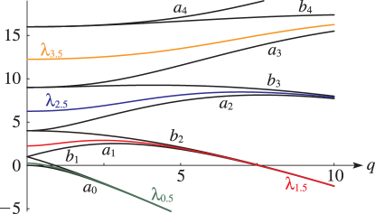
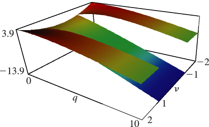
►As functions of , and can be continued analytically in the complex -plane.
The only singularities are algebraic branch points, with and finite at these points.
…The normal values are simple roots of the corresponding equations (28.2.21) and (28.2.22).
…
►
…
Arscott and Khabaza (1962) tabulates the coefficients of the polynomials in
Table 29.12.1 (normalized so that the numerically largest
coefficient is unity, i.e. monic polynomials), and the corresponding eigenvalues
for
, . Equations from §29.6 can be used
to transform to the normalization adopted in this chapter. Precision is 6S.
…
►Initial approximations to the eigenvalues can be found, for example, from the asymptotic expansions supplied in §29.7(i).
…
►A third method is to approximate eigenvalues and Fourier coefficients of Lamé functions by eigenvalues and eigenvectors of finite matrices using the methods of §§3.2(vi) and 3.8(iv).
…
►
§29.20(ii) Lamé Polynomials
►The eigenvalues corresponding to Lamé polynomials are computed from eigenvalues of the finite tridiagonal matrices given in §29.15(i), using methods described in §3.2(vi) and Ritter (1998).
…
…
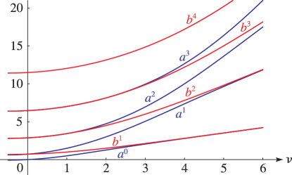
►If is not an integer, then (29.2.1) is unstable iff or lies in one of the closed intervals with endpoints and , .
If is a nonnegative integer, then (29.2.1) is unstable iff or for some .
►Methods for computing the eigenvalues
, , and , defined in §§28.2(v) and 28.12(i), include:
…
►
(d)
Solution of the matrix eigenvalue problem for each of the five infinite
matrices that correspond to the linear algebraic equations (28.4.5)–(28.4.8)
and (28.14.4). See
Zhang and Jin (1996, pp. 479–482) and §3.2(iv).
Asymptotic approximations by zeros of orthogonal polynomials of increasing degree.
See Volkmer (2008). This method also applies to eigenvalues of the
Whittaker–Hill equation (§28.31(i)) and eigenvalues of Lamé
functions (§29.3(i)).
…
►Also, once the eigenvalues
, , and have been computed the following methods are applicable:
…
►Leading terms of the power series for and for are:
…
►The coefficients of the power series of , and also , are the same until the terms in and , respectively.
…
►Higher coefficients in the foregoing series can be found by equating coefficients in the following continued-fraction equations:
…
►Here for , for , and for and .
…
 ►
►
 ►
►
 ►
►
 ►
►
 ►
►
