Whittaker equation

SearchAdvancedHelp

(0.002 seconds)

21—30 of 60 matching pages

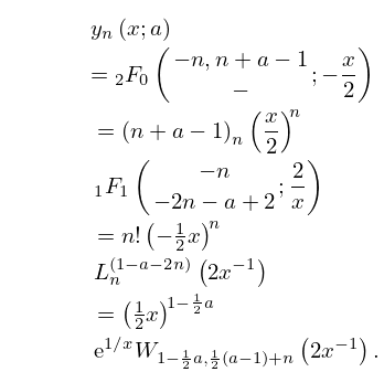
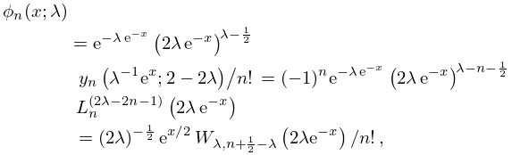
21: 18.34 Bessel Polynomials

… ►

18.34.1 $$y_n(x;a)={}_2{}^{}F_0^{}(\genfrac{}{}{0pt}{}{-n,n+a-1}{-};-\frac{x}{2})={\left(n+a-1\right)}_n{\left(\frac{x}{2}\right)}^n{}_1{}^{}F_1^{}(\genfrac{}{}{0pt}{}{-n}{-2n-a+2};\frac{2}{x})=n!{\left(-\frac{1}{2}x\right)}^n{L}_n^{(1-a-2n)}\left(2x^{-1}\right)={\left(\frac{1}{2}x\right)}^{1-\frac{1}{2}a}{\mathrm{e}}^{1/x}{W}_{1-\frac{1}{2}a,\frac{1}{2}(a-1)+n}\left(2x^{-1}\right).$$

ⓘ

Defines:

$y_n(x;a)$: Bessel polynomial

Symbols:

${}_p{}^{}F_q^{}(a_1,\mathrm{\dots },a_p;b_1,\mathrm{\dots },b_q;z)$ or ${}_p{}^{}F_q^{}(\genfrac{}{}{0pt}{}{a_1,\mathrm{\dots },a_p}{b_1,\mathrm{\dots },b_q};z)$: alternatively ${}_p{}^{}F_q^{}(𝐚;𝐛;z)$ or ${}_p{}^{}F_q^{}(\genfrac{}{}{0pt}{}{𝐚}{𝐛};z)$
generalized hypergeometric function, ${}_1{}^{}F_1^{}(a;b;z)$: $=M(a,b,z)$ notation for the Kummer confluent hypergeometric function, $L_n^{(\alpha )}\left(x\right)$: Laguerre (or generalized Laguerre) polynomial, ${\left(a\right)}_n$: Pochhammer’s symbol (or shifted factorial), $W_{\kappa ,\mu }\left(z\right)$: Whittaker confluent hypergeometric function, $\mathrm{e}$: base of natural logarithm, $!$: factorial (as in $n!$), $n$: nonnegative integer and $x$: real variable

Proved:

Grosswald (1978, p.38, Theorem 1); Combine (18.5.12) and items (i), (v), (vii) of the mentioned theorem for $b=2$(proved)

Referenced by:

(18.34.2), (18.34.7_1), §18.34(i), §18.34(i), Erratum (V1.2.0) for Equation (18.34.1)

Permalink:

http://dlmf.nist.gov/18.34.E1

Encodings:

pMML, png, TeX

Addition (effective with 1.2.0):

This equation was updated to include the definition of Bessel polynomials in terms of Laguerre polynomials and the Whittaker confluent hypergeometric function.

See also:

Annotations for §18.34(i), §18.34 and Ch.18

… ►

18.34.7_1 $${\varphi }_n(x;\lambda )={\mathrm{e}}^{-\lambda {\mathrm{e}}^{-x}}{\left(2\lambda {\mathrm{e}}^{-x}\right)}^{\lambda -\frac{1}{2}}{y}_n({\lambda }^{-1}{\mathrm{e}}^x;2-2\lambda )/n!={(-1)}^n{\mathrm{e}}^{-\lambda {\mathrm{e}}^{-x}}{\left(2\lambda {\mathrm{e}}^{-x}\right)}^{\lambda -n-\frac{1}{2}}{L}_n^{(2\lambda -2n-1)}\left(2\lambda {\mathrm{e}}^{-x}\right)={(2\lambda )}^{-\frac{1}{2}}{\mathrm{e}}^{x/2}{W}_{\lambda ,n+\frac{1}{2}-\lambda }\left(2\lambda {\mathrm{e}}^{-x}\right)/n!,$$ $n=0,1,\mathrm{\dots },N=\lceil \lambda -\frac{3}{2}\rceil$, $\lambda >\frac{1}{2}$,

ⓘ

Symbols:

$y_n(x;a)$: Bessel polynomial, $L_n^{(\alpha )}\left(x\right)$: Laguerre (or generalized Laguerre) polynomial, $W_{\kappa ,\mu }\left(z\right)$: Whittaker confluent hypergeometric function, $\lceil x\rceil$: ceiling of $x$ , $\mathrm{e}$: base of natural logarithm, $!$: factorial (as in $n!$), $N$: positive integer, $n$: nonnegative integer and $x$: real variable

Proof sketch:

The second and third equality follow from (18.34.1).

Referenced by:

(18.34.7_2), (18.34.7_3), §18.34(iii), (18.39.17), (18.39.18), §18.39(i), Erratum (V1.2.0) Section 18.34

Permalink:

http://dlmf.nist.gov/18.34.E7_1

Encodings:

pMML, png, TeX

Addition (effective with 1.2.0):

This equation was added.

See also:

Annotations for §18.34(iii), §18.34 and Ch.18

…

22: 23.21 Physical Applications

… ►See, for example, Lawden (1989, Chapter 7) and Whittaker (1964, Chapters 4–6). ►

§23.21(ii) Nonlinear Evolution Equations

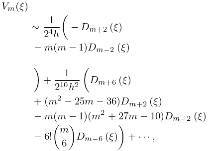
►Airault et al. (1977) applies the function $\mathrm{\wp }$ to an integrable classical many-body problem, and relates the solutions to nonlinear partial differential equations. For applications to soliton solutions of the Korteweg–de Vries (KdV) equation see McKean and Moll (1999, p. 91), Deconinck and Segur (2000), and Walker (1996, §8.1). …

23: 28.8 Asymptotic Expansions for Large $q$

… ►

28.8.5 $$V_m(\xi )\sim \frac{1}{2^{4}h}\left(-D_{m+2}\left(\xi \right)-m(m-1)D_{m-2}\left(\xi \right)\right)+\frac{1}{2^{10}{h}^2}\left(D_{m+6}\left(\xi \right)+(m^2-25m-36)D_{m+2}\left(\xi \right)-m(m-1)(m^2+27m-10)D_{m-2}\left(\xi \right)-6!\left(\genfrac{}{}{0.0pt}{}{m}{6}\right)D_{m-6}\left(\xi \right)\right)+\mathrm{\cdots },$$

ⓘ

Defines:

$V_m(\xi )$: function (locally)

Symbols:

$D_{\nu }\left(z\right)$: parabolic cylinder function, $\sim$: Poincaré asymptotic expansion, $\left(\genfrac{}{}{0.0pt}{}{m}{n}\right)$: binomial coefficient, $!$: factorial (as in $n!$), $m$: integer, $h$: parameter and $\xi$: variable

A&S Ref:

20.9.18 (in slightly different form)

Referenced by:

Erratum (V1.0.16) for Equation (28.8.5)

Permalink:

http://dlmf.nist.gov/28.8.E5

Encodings:

pMML, png, TeX

Error (effective with 1.0.16):

Originally the $-$ in front of the $6!$ was given incorrectly as $+$.

Suggested 2017-02-02 by Daniel Karlsson

See also:

Annotations for §28.8(ii), §28.8 and Ch.28

…

24: 33.14 Definitions and Basic Properties

… ►

33.14.14 $${\varphi }_{n,\mathrm{\ell }}(r)={(-1)}^{\mathrm{\ell }+1+n}{(2/n^3)}^{1/2}s(-1/n^2,\mathrm{\ell };r)=\frac{{(-1)}^{\mathrm{\ell }+1+n}}{n^{\mathrm{\ell }+2}}{\left(\frac{(n-\mathrm{\ell }-1)!}{(n+\mathrm{\ell })!}\right)}^{1/2}{(2r)}^{\mathrm{\ell }+1}{\mathrm{e}}^{-r/n}{L}_{n-\mathrm{\ell }-1}^{(2\mathrm{\ell }+1)}\left(2r/n\right)$$

ⓘ

Defines:

${\varphi }_{n,\mathrm{\ell }}(r)$: function (locally)

Symbols:

$s(ϵ,\mathrm{\ell };r)$: regular Coulomb function, $L_n^{(\alpha )}\left(x\right)$: Laguerre (or generalized Laguerre) polynomial, $\mathrm{e}$: base of natural logarithm, $!$: factorial (as in $n!$), $\mathrm{\ell }$: nonnegative integer and $r$: real variable

Referenced by:

(33.14.14), (33.14.15), §33.14(iv), §33.22(v), Erratum (V1.0.24) for Equation (33.14.15), Erratum (V1.0.24) for Subsection 33.14(iv)

Permalink:

http://dlmf.nist.gov/33.14.E14

Encodings:

pMML, png, TeX

Addition (effective with 1.0.24):

For the second equation in (33.14.14) first, via (33.14.9) and (33.14.4), express ${\varphi }_{n,\mathrm{\ell }}(r)$ in terms of Whittaker functions and then use (13.18.17).

See also:

Annotations for §33.14(iv), §33.14 and Ch.33

…

25: 33.22 Particle Scattering and Atomic and Molecular Spectra

… ►

§33.22(i) Schrödinger Equation

… ►

§33.22(iv) Klein–Gordon and Dirac Equations

… ►For bound-state problems only the exponentially decaying solution is required, usually taken to be the Whittaker function $W_{-\eta ,\mathrm{\ell }+\frac{1}{2}}\left(2\rho \right)$. … ►

§33.22(vi) Solutions Inside the Turning Point

… ►

Solution of relativistic Coulomb equations. See for example Cooper et al. (1979) and Barnett (1981b).

…

26: 28.1 Special Notation

… ► ►►►

$m,n$	integers.
…
$a,q,h$	real or complex parameters of Mathieu’s equation with $q=h^2$.
…

… ► ►►

${\mathrm{ce}}_{\nu }(z,q)$,

${\mathrm{se}}_{\nu }(z,q)$,

${\mathrm{fe}}_n(z,q)$,

${\mathrm{ge}}_n(z,q)$,

${\mathrm{me}}_{\nu }(z,q)$,

… ►The eigenvalues of Mathieu’s equation are denoted by … ►

${\lambda }_{\nu }\left(q\right).$

… ►

Table 28.1.1: Notations for parameters in Mathieu’s equation.

► ►►

Reference	$a$	$q$
…

►

…

27: Bibliography N

… ►

Toda equation and its solutions in special functions. J. Phys. Soc. Japan 65 (6), pp. 1589–1597.

ⓘ

External Links:

ISSN 0031-9015, Document, MathReview, ZentralBlatt

Referenced by:

§18.38(ii).

Encodings:

BibTeX

… ►

Confluent hypergeometric equations and related solvable potentials in quantum mechanics. J. Math. Phys. 41 (12), pp. 7964–7996.

ⓘ

External Links:

ISSN 0022-2488, Document, MathReview, ZentralBlatt

Referenced by:

§13.28(i).

Encodings:

BibTeX

… ►

Uniform Asymptotic Approximations of Solutions of Second-order Linear Differential Equations, with a Coalescing Simple Turning Point and Simple Pole. Ph.D. Thesis, University of Maryland, College Park, MD.

ⓘ

Referenced by:

§2.8(vi).

Encodings:

BibTeX

… ►

Solving equations exactly. J. Res. Nat. Bur. Standards Sect. B 71B, pp. 171–179.

ⓘ

External Links:

MathReview, ZentralBlatt

Referenced by:

§27.15.

Encodings:

BibTeX

… ►

Evaluation of negative energy Coulomb (Whittaker) functions. Comput. Phys. Comm. 159 (1), pp. 55–62.

ⓘ

Notes:

Double-precision Fortran-90 code.

External Links:

Document, Code

Referenced by:

§33.23(vi), 8th item.

Encodings:

BibTeX

…

28: 2.8 Differential Equations with a Parameter

§2.8 Differential Equations with a Parameter

… ►The transformed equation has the form …In Case III the approximating equation is … ►The transformed differential equation is … ►For examples of uniform asymptotic approximations in terms of Whittaker functions with fixed second parameter see §18.15(i) and §28.8(iv). …

29: 23.22 Methods of Computation

… ►Suppose that the invariants $g_2=c$, $g_3=d$, are given, for example in the differential equation (23.3.10) or via coefficients of an elliptic curve (§23.20(ii)). The determination of suitable generators $2{\omega }_1$ and $2{\omega }_3$ is the classical inversion problem (Whittaker and Watson (1927, §21.73), McKean and Moll (1999, §2.12); see also §20.9(i) and McKean and Moll (1999, §2.16)). … ►

In the general case, given by $cd\ne 0$, we compute the roots $\alpha$, $\beta$, $\gamma$, say, of the cubic equation $4t^3-ct-d=0$; see §1.11(iii). These roots are necessarily distinct and represent $e_1$, $e_2$, $e_3$ in some order.

If $c$ and $d$ are real, and the discriminant is positive, that is $c^3-27d^2>0$, then $e_1$, $e_2$, $e_3$ can be identified via (23.5.1), and $k^2$, $k_{}^{\prime }{}_{}{}^2$ obtained from (23.6.16).

If , or $c$ and $d$ are not both real, then we label $\alpha$, $\beta$, $\gamma$ so that the triangle with vertices $\alpha$, $\beta$, $\gamma$ is positively oriented and $[\alpha ,\gamma ]$ is its longest side (chosen arbitrarily if there is more than one). In particular, if $\alpha$, $\beta$, $\gamma$ are collinear, then we label them so that $\beta$ is on the line segment $(\alpha ,\gamma )$. In consequence, $k^2=(\beta -\gamma )/(\alpha -\gamma )$, $k_{}^{\prime }{}_{}{}^2=(\alpha -\beta )/(\alpha -\gamma )$ satisfy $\mathrm{\Im }{k}^2\ge 0\ge \mathrm{\Im }k_{}^{\prime }{}_{}{}^2$ (with strict inequality unless $\alpha$, $\beta$, $\gamma$ are collinear); also $|k^2|$, $|k_{}^{\prime }{}_{}{}^2|\le 1$.

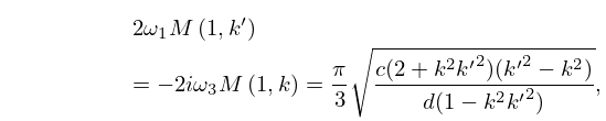
Finally, on taking the principal square roots of $k^2$ and $k_{}^{\prime }{}_{}{}^2$ we obtain values for $k$ and $k^{\prime }$ that lie in the 1st and 4th quadrants, respectively, and $2{\omega }_1$, $2{\omega }_3$ are given by

23.22.1 $$2{\omega }_{1}M(1,k^{\prime })=-2\mathrm{i}{\omega }_{3}M(1,k)=\frac{\pi }{3}\sqrt{\frac{c(2+k^{2}k_{}^{\prime }{}_{}{}^2)(k_{}^{\prime }{}_{}{}^2-k^2)}{d(1-k^{2}k_{}^{\prime }{}_{}{}^2)}},$$

ⓘ

Symbols:

$M(a,g)$: arithmetic-geometric mean, $\pi$: the ratio of the circumference of a circle to its diameter, $\mathrm{i}$: imaginary unit, ${\omega }_1$, ${\omega }_3$, ${\omega }_2=-{\omega }_1-{\omega }_3$: lattice generators, $k$: modulus and $k^{\prime }$: complementary modulus

Proof sketch:

Combine (23.6.16), (23.6.17), (22.20.6), (23.3.5)–(23.3.7), and use analytical continuation.

Referenced by:

§23.22(ii)

Permalink:

http://dlmf.nist.gov/23.22.E1

Encodings:

pMML, png, TeX

See also:

Annotations for §23.22(ii), §23.22(ii), §23.22 and Ch.23

where $M$ denotes the arithmetic-geometric mean (see §§19.8(i) and 22.20(ii)). This process yields 2 possible pairs ($2{\omega }_1$, $2{\omega }_3$), corresponding to the 2 possible choices of the square root.

…

30: 22.19 Physical Applications

… ►Classical motion in one dimension is described by Newton’s equation … ►

§22.19(iii) Nonlinear ODEs and PDEs

… ► … ►Elementary discussions of this topic appear in Lawden (1989, §5.7), Greenhill (1959, pp. 101–103), and Whittaker (1964, Chapter VI). … ►Whittaker (1964, Chapter IV) enumerates the complete class of one-body classical mechanical problems that are solvable this way. …