Weber%E2%80%93Schafheitlin%20discontinuous%20integrals

SearchAdvancedHelp

(0.004 seconds)

11—20 of 508 matching pages

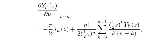
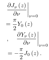
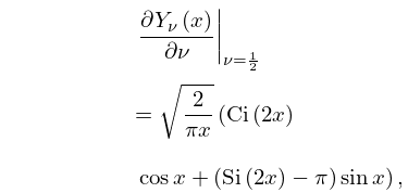
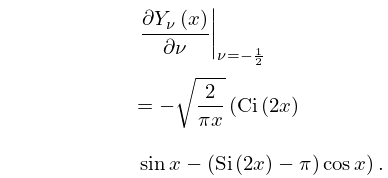
11: 10.15 Derivatives with Respect to Order

… ►

10.15.4 $${\frac{\partial Y_{\nu }\left(z\right)}{\partial \nu }|}_{\nu =n}=-\frac{\pi }{2}{J}_n\left(z\right)+\frac{n!}{2{(\frac{1}{2}z)}^n}\sum _{k=0}^{n-1}\frac{{(\frac{1}{2}z)}^k{Y}_k\left(z\right)}{k!(n-k)},$$

ⓘ

Symbols:

$J_{\nu }\left(z\right)$: Bessel function of the first kind, $Y_{\nu }\left(z\right)$: Bessel function of the second kind, $\pi$: the ratio of the circumference of a circle to its diameter, $!$: factorial (as in $n!$), $\frac{\partial f}{\partial x}$: partial derivative of $f$ with respect to $x$ , $\partial x$: partial differential of $x$ , $n$: integer, $k$: nonnegative integer, $z$: complex variable and $\nu$: complex parameter

A&S Ref:

9.1.67

Permalink:

http://dlmf.nist.gov/10.15.E4

Encodings:

pMML, png, TeX

See also:

Annotations for §10.15, §10.15 and Ch.10

►

10.15.5 $${\frac{\partial J_{\nu }\left(z\right)}{\partial \nu }|}_{\nu =0}=\frac{\pi }{2}{Y}_0\left(z\right),{\frac{\partial Y_{\nu }\left(z\right)}{\partial \nu }|}_{\nu =0}=-\frac{\pi }{2}{J}_0\left(z\right).$$

ⓘ

Symbols:

$J_{\nu }\left(z\right)$: Bessel function of the first kind, $Y_{\nu }\left(z\right)$: Bessel function of the second kind, $\pi$: the ratio of the circumference of a circle to its diameter, $\frac{\partial f}{\partial x}$: partial derivative of $f$ with respect to $x$ , $\partial x$: partial differential of $x$ , $z$: complex variable and $\nu$: complex parameter

A&S Ref:

9.1.68

Referenced by:

§10.15, §10.38

Permalink:

http://dlmf.nist.gov/10.15.E5

Encodings:

pMML, png, TeX

See also:

Annotations for §10.15, §10.15 and Ch.10

… ►For the notations $\mathrm{Ci}$ and $\mathrm{Si}$ see §6.2(ii). … ►

10.15.8 $${\frac{\partial Y_{\nu }\left(x\right)}{\partial \nu }|}_{\nu =\frac{1}{2}}=\sqrt{\frac{2}{\pi x}}\left(\mathrm{Ci}\left(2x\right)\cos x+\left(\mathrm{Si}\left(2x\right)-\pi \right)\sin x\right),$$

ⓘ

Symbols:

$Y_{\nu }\left(z\right)$: Bessel function of the second kind, $\pi$: the ratio of the circumference of a circle to its diameter, $\cos z$: cosine function, $\mathrm{Ci}\left(z\right)$: cosine integral, $\frac{\partial f}{\partial x}$: partial derivative of $f$ with respect to $x$ , $\partial x$: partial differential of $x$ , $\sin z$: sine function, $\mathrm{Si}\left(z\right)$: sine integral, $x$: real variable and $\nu$: complex parameter

A&S Ref:

10.1.43 (corrected)

Referenced by:

§10.15

Permalink:

http://dlmf.nist.gov/10.15.E8

Encodings:

pMML, png, TeX

See also:

Annotations for §10.15, §10.15 and Ch.10

►

10.15.9 $${\frac{\partial Y_{\nu }\left(x\right)}{\partial \nu }|}_{\nu =-\frac{1}{2}}=-\sqrt{\frac{2}{\pi x}}\left(\mathrm{Ci}\left(2x\right)\sin x-\left(\mathrm{Si}\left(2x\right)-\pi \right)\cos x\right).$$

ⓘ

Symbols:

$Y_{\nu }\left(z\right)$: Bessel function of the second kind, $\pi$: the ratio of the circumference of a circle to its diameter, $\cos z$: cosine function, $\mathrm{Ci}\left(z\right)$: cosine integral, $\frac{\partial f}{\partial x}$: partial derivative of $f$ with respect to $x$ , $\partial x$: partial differential of $x$ , $\sin z$: sine function, $\mathrm{Si}\left(z\right)$: sine integral, $x$: real variable and $\nu$: complex parameter

A&S Ref:

10.1.44 (corrected)

Referenced by:

§10.15, Ch.10

Permalink:

http://dlmf.nist.gov/10.15.E9

Encodings:

pMML, png, TeX

See also:

Annotations for §10.15, §10.15 and Ch.10

…

12: 11.15 Approximations

… ►

Luke (1975, pp. 416–421) gives Chebyshev-series expansions for ${𝐇}_n\left(x\right)$, ${𝐋}_n\left(x\right)$, $0\le \left|x\right|\le 8$, and ${𝐇}_n\left(x\right)-Y_n\left(x\right)$, $x\ge 8$, for $n=0,1$; ${\int }_0^x{t}^{-m}{𝐇}_0\left(t\right)dt$, ${\int }_0^x{t}^{-m}{𝐋}_0\left(t\right)dt$, $0\le \left|x\right|\le 8$, $m=0,1$ and ${\int }_0^x({𝐇}_0\left(t\right)-Y_0\left(t\right))dt$, ${\int }_x^{\mathrm{\infty }}{t}^{-1}({𝐇}_0\left(t\right)-Y_0\left(t\right))dt$, $x\ge 8$; the coefficients are to 20D.

… ►

Newman (1984) gives polynomial approximations for ${𝐇}_n\left(x\right)$ for $n=0,1$, $0\le x\le 3$, and rational-fraction approximations for ${𝐇}_n\left(x\right)-Y_n\left(x\right)$ for $n=0,1$, $x\ge 3$. The maximum errors do not exceed 1.2×10⁻⁸ for the former and 2.5×10⁻⁸ for the latter.

13: 10.2 Definitions

… ►

Bessel Function of the Second Kind (Weber’s Function)

… ►Whether or not $\nu$ is an integer $Y_{\nu }\left(z\right)$ has a branch point at $z=0$. … ►Except in the case of $J_{\pm n}\left(z\right)$, the principal branches of $J_{\nu }\left(z\right)$ and $Y_{\nu }\left(z\right)$ are two-valued and discontinuous on the cut $\mathrm{ph}z=\pm \pi$; compare §4.2(i). ►Both $J_{\nu }\left(z\right)$ and $Y_{\nu }\left(z\right)$ are real when $\nu$ is real and $\mathrm{ph}z=0$. ►For fixed $z$ $(\ne 0)$ each branch of $Y_{\nu }\left(z\right)$ is entire in $\nu$. …

14: 11.1 Special Notation

§11.1 Special Notation

… ►For the functions $J_{\nu }\left(z\right)$, $Y_{\nu }\left(z\right)$, $H_{\nu }^{(1)}\left(z\right)$, $H_{\nu }^{(2)}\left(z\right)$, $I_{\nu }\left(z\right)$, and $K_{\nu }\left(z\right)$ see §§10.2(ii), 10.25(ii). ►The functions treated in this chapter are the Struve functions ${𝐇}_{\nu }\left(z\right)$ and ${𝐊}_{\nu }\left(z\right)$, the modified Struve functions ${𝐋}_{\nu }\left(z\right)$ and ${𝐌}_{\nu }\left(z\right)$, the Lommel functions $s_{\mu ,\nu }\left(z\right)$ and $S_{\mu ,\nu }\left(z\right)$, the Anger function ${𝐉}_{\nu }\left(z\right)$, the Weber function ${𝐄}_{\nu }\left(z\right)$, and the associated Anger–Weber function ${𝐀}_{\nu }\left(z\right)$.

15: Bibliography H

… ►

The Laplace transform for expressions that contain a probability function. Bul. Akad. Štiince RSS Moldoven. 1973 (2), pp. 78–80, 93 (Russian).

ⓘ

External Links:

MathReview (L. Berg)

Referenced by:

§7.14(iii).

Encodings:

BibTeX

… ►

Integrals containing the Fresnel functions $S(x)$ and $C(x)$ . Bul. Akad. Štiince RSS Moldoven. 1975 (3), pp. 48–60, 93 (Russian).

ⓘ

External Links:

MathReview (J. Kaczmarski)

Referenced by:

§7.14(iii).

Encodings:

BibTeX

… ►

Integrals that contain a probability function of complicated arguments. Bul. Akad. Štiince RSS Moldoven. 1976 (1), pp. 80–84, 96 (Russian).

ⓘ

External Links:

MathReview (V. L. Makarov)

Referenced by:

§7.14(iii).

Encodings:

BibTeX

… ►

Some properties and applications of the repeated integrals of the error function. Proc. Manchester Lit. Philos. Soc. 80, pp. 85–102.

ⓘ

External Links:

ZentralBlatt

Referenced by:

§7.18(iii), §7.18(iv), §7.18(v), §7.18(vi).

Encodings:

BibTeX

… ►

Diffraction and Weber functions. SIAM J. Appl. Math. 57 (6), pp. 1702–1715.

ⓘ

External Links:

ISSN 0036-1399, Document, MathReview, ZentralBlatt

Referenced by:

§12.13(ii), §12.17.

Encodings:

BibTeX

…

16: 6.2 Definitions and Interrelations

… ►

§6.2(i) Exponential and Logarithmic Integrals

… ► … ►The logarithmic integral is defined by … ►

§6.2(ii) Sine and Cosine Integrals

… ► …

17: Bibliography

… ►

Regular and irregular Coulomb wave functions expressed in terms of Bessel-Clifford functions. J. Math. Physics 33, pp. 111–116.

ⓘ

External Links:

MathReview (E. Weber), ZentralBlatt

Referenced by:

§33.9(ii).

Encodings:

BibTeX

… ►

Algorithm 511: CDC 6600 subroutines IBESS and JBESS for Bessel functions $I_{\nu }(x)$ and $J_{\nu }(x)$, $x\ge 0$, $\nu \ge 0$ . ACM Trans. Math. Software 3 (1), pp. 93–95.

ⓘ

Notes:

Single-precision Fortran, maximum accuracy 16S.

External Links:

ISSN 0098-3500, Document, Companion paper. Erratum. GAMS (module 511; package TOMS)

Referenced by:

1st item, 1st item.

Encodings:

BibTeX

… ►

Algorithm 683: A portable FORTRAN subroutine for exponential integrals of a complex argument. ACM Trans. Math. Software 16 (2), pp. 178–182.

ⓘ

Notes:

Double- and single-precision Fortran, maximum accuracy 18S or 14S.

External Links:

ISSN 0098-3500, Document, GAMS (module 683; package TOMS), MathReview, ZentralBlatt

Referenced by:

1st item, 1st item.

Encodings:

BibTeX

… ►

Mathematical Methods for Physicists. 6th edition, Elsevier, Oxford.

ⓘ

External Links:

ISBN 0-12-059876-0;0-12-088584-0, MathReview, ZentralBlatt

Referenced by:

§1.17(ii), §1.17(iii).

Encodings:

BibTeX

… ►

Quadratic differentials and asymptotics of Laguerre polynomials with varying complex parameters. J. Math. Anal. Appl. 416 (1), pp. 52–80.

ⓘ

External Links:

ISSN 0022-247X, Document, Link, MathReview (Vivek Sahai), ZentralBlatt

Referenced by:

§18.15(vi), §18.15(vi).

Encodings:

BibTeX

…

18: 10.24 Functions of Imaginary Order

… ►and ${\tilde{J}}_{\nu }\left(x\right)$, ${\tilde{Y}}_{\nu }\left(x\right)$ are linearly independent solutions of (10.24.1): … ►In consequence of (10.24.6), when $x$ is large ${\tilde{J}}_{\nu }\left(x\right)$ and ${\tilde{Y}}_{\nu }\left(x\right)$ comprise a numerically satisfactory pair of solutions of (10.24.1); compare §2.7(iv). … ►For graphs of ${\tilde{J}}_{\nu }\left(x\right)$ and ${\tilde{Y}}_{\nu }\left(x\right)$ see §10.3(iii). ►For mathematical properties and applications of ${\tilde{J}}_{\nu }\left(x\right)$ and ${\tilde{Y}}_{\nu }\left(x\right)$, including zeros and uniform asymptotic expansions for large $\nu$, see Dunster (1990a). In this reference ${\tilde{J}}_{\nu }\left(x\right)$ and ${\tilde{Y}}_{\nu }\left(x\right)$ are denoted respectively by $F_{\mathrm{i}\nu }(x)$ and $G_{\mathrm{i}\nu }(x)$. …

19: 10.1 Special Notation

… ►The main functions treated in this chapter are the Bessel functions $J_{\nu }\left(z\right)$, $Y_{\nu }\left(z\right)$; Hankel functions $H_{\nu }^{(1)}\left(z\right)$, $H_{\nu }^{(2)}\left(z\right)$; modified Bessel functions $I_{\nu }\left(z\right)$, $K_{\nu }\left(z\right)$; spherical Bessel functions ${𝗃}_n\left(z\right)$, ${𝗒}_n\left(z\right)$, ${𝗁}_n^{(1)}\left(z\right)$, ${𝗁}_n^{(2)}\left(z\right)$; modified spherical Bessel functions ${𝗂}_n^{(1)}\left(z\right)$, ${𝗂}_n^{(2)}\left(z\right)$, ${𝗄}_n\left(z\right)$; Kelvin functions ${\mathrm{ber}}_{\nu }\left(x\right)$, ${\mathrm{bei}}_{\nu }\left(x\right)$, ${\ker }_{\nu }\left(x\right)$, ${\mathrm{kei}}_{\nu }\left(x\right)$. … ►A common alternative notation for $Y_{\nu }\left(z\right)$ is $N_{\nu }(z)$. … ►For older notations see British Association for the Advancement of Science (1937, pp. xix–xx) and Watson (1944, Chapters 1–3).

20: 10.58 Zeros

… ►

$b_{n,m}=y_{n+\frac{1}{2},m},$

… ►

${𝗒}_n^{\prime }\left(b_{n,m}\right)=\sqrt{{\displaystyle \frac{\pi }{2y_{n+\frac{1}{2},m}}}}{Y}_{n+\frac{1}{2}}^{\prime }\left(y_{n+\frac{1}{2},m}\right).$

…