SL(2,Z)

(0.002 seconds)

11—20 of 803 matching pages

11: 10.44 Sums

… ►

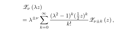
10.44.1

\mathscr{Z}_{\nu}\left(\lambda z\right)=\lambda^{\pm\nu}\sum_{k=0}^{\infty}% \frac{(\lambda^{2}-1)^{k}(\frac{1}{2}z)^{k}}{k!}\mathscr{Z}_{\nu\pm k}\left(z% \right),

|\lambda^{2}-1|<1

ⓘ

Symbols:: $!$ : factorial (as in $n!$ ), $\mathscr{Z}_{\NVar{\nu}}\left(\NVar{z}\right)$ : modified cylinder function, $k$ : nonnegative integer, $z$ : complex variable and $\nu$ : complex parameter
A&S Ref:: 9.6.51
Referenced by:: §10.44(i), §10.66
Permalink:: http://dlmf.nist.gov/10.44.E1
Encodings:: pMML, png, TeX
See also:: Annotations for §10.44(i), §10.44 and Ch.10

►If

\mathscr{Z}=I

and the upper signs are taken, then the restriction on

\lambda

is unnecessary. … ►

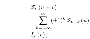
10.44.3

\mathscr{Z}_{\nu}\left(u\pm v\right)=\sum_{k=-\infty}^{\infty}(\pm 1)^{k}% \mathscr{Z}_{\nu+k}\left(u\right)I_{k}\left(v\right),

|v|<|u|

ⓘ

Symbols:: $I_{\NVar{\nu}}\left(\NVar{z}\right)$ : modified Bessel function of the first kind, $\mathscr{Z}_{\NVar{\nu}}\left(\NVar{z}\right)$ : modified cylinder function, $k$ : nonnegative integer and $\nu$ : complex parameter
Permalink:: http://dlmf.nist.gov/10.44.E3
Encodings:: pMML, png, TeX
See also:: Annotations for §10.44(ii), §10.44(ii), §10.44 and Ch.10

►The restriction

|v|<|u|

is unnecessary when

\mathscr{Z}=I

and

\nu

is an integer. … ►

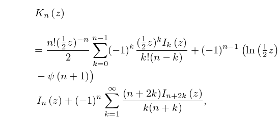
10.44.6

K_{n}\left(z\right)=\frac{n!(\tfrac{1}{2}z)^{-n}}{2}\sum_{k=0}^{n-1}(-1)^{k}% \frac{(\tfrac{1}{2}z)^{k}I_{k}\left(z\right)}{k!(n-k)}+(-1)^{n-1}\left(\ln% \left(\tfrac{1}{2}z\right)-\psi\left(n+1\right)\right)I_{n}\left(z\right)+(-1)% ^{n}\sum_{k=1}^{\infty}\frac{(n+2k)I_{n+2k}\left(z\right)}{k(n+k)},

ⓘ

Symbols:: $\psi\left(\NVar{z}\right)$ : psi (or digamma) function, $!$ : factorial (as in $n!$ ), $I_{\NVar{\nu}}\left(\NVar{z}\right)$ : modified Bessel function of the first kind, $K_{\NVar{\nu}}\left(\NVar{z}\right)$ : modified Bessel function of the second kind, $\ln\NVar{z}$ : principal branch of logarithm function, $n$ : integer, $k$ : nonnegative integer and $z$ : complex variable
A&S Ref:: 9.6.53
Permalink:: http://dlmf.nist.gov/10.44.E6
Encodings:: pMML, png, TeX
See also:: Annotations for §10.44(iii), §10.44 and Ch.10

…

12: 18.39 Applications in the Physical Sciences

… ►This is also the normalization and notation of Chapter 33 for

Z=1

, and the notation of Weinberg (2013, Chapter 2). … ►Thus the

c_{N}(x)=P^{(l+1)}_{N}\left(x;\frac{2Z}{s},-\frac{2Z}{s}\right)

and the eigenvalues …are determined by the

N

zeros,

x^{N}_{i}

of the Pollaczek polynomial

P^{(l+1)}_{N}\left(x;\frac{2Z}{s},-\frac{2Z}{s}\right)

. … ►The polynomials

P^{(l+1)}_{N}\left(x;\frac{2Z}{s},-\frac{2Z}{s}\right)

, for both positive and negative

Z

, define the Coulomb–Pollaczek polynomials (CP OP’s in what follows), see Yamani and Reinhardt (1975, Appendix B, and §IV). … ►Note that violation of the Favard inequality,

l+1+(2Z/s)>0,

possible when

Z<0

, results in a zero or negative weight function. …

13: 19.19 Taylor and Related Series

… ►For

N=0,1,2,\dots

define the homogeneous hypergeometric polynomial … ►If

n=2

, then (19.19.3) is a Gauss hypergeometric series (see (19.25.43) and (15.2.1)). … ►and define the

n

-tuple

\mathbf{\tfrac{1}{2}}=(\tfrac{1}{2},\dots,\tfrac{1}{2})

. … ►The number of terms in

T_{N}

can be greatly reduced by using variables

\mathbf{Z}=\boldsymbol{{1}}-(\mathbf{z}/A)

with

A

chosen to make

E_{1}(\mathbf{Z})=0

. … ►

19.19.7

R_{-a}\left(\boldsymbol{{\tfrac{1}{2}}};\mathbf{z}\right)=A^{-a}\sum_{N=0}^{% \infty}\frac{{\left(a\right)_{N}}}{{\left(\tfrac{1}{2}n\right)_{N}}}T_{N}(% \boldsymbol{{\tfrac{1}{2}}},\mathbf{Z}),

ⓘ

Symbols:: $R_{\NVar{-a}}\left(\NVar{b_{1}},\dots,\NVar{b_{n}};\NVar{z_{1}},\dots,\NVar{z_% {n}}\right)$ or $R_{\NVar{-a}}\left(\NVar{\mathbf{b}};\NVar{\mathbf{z}}\right)$ : multivariate hypergeometric function, ${\left(\NVar{a}\right)_{\NVar{n}}}$ : Pochhammer’s symbol (or shifted factorial), $n$ : nonnegative integer, $N$ : nonnegative integer, $T_{N}(\mathbf{b},\mathbf{z})$ : polynomial, $\mathbf{Z}$ : variable and $A$
Referenced by:: §19.15, §19.36(i), §19.36(i), §19.36(i)
Permalink:: http://dlmf.nist.gov/19.19.E7
Encodings:: pMML, png, TeX
See also:: Annotations for §19.19 and Ch.19

…

14: 22.16 Related Functions

… ►With

q

as in (22.2.1) and

\zeta=\pi x/(2K)

, … ►In Equations (22.16.24)–(22.16.26),

-2K<x<2K

. … ►where

\xi=x/{\theta_{3}}^{2}\left(0,q\right)

. … ►(Sometimes in the literature

\mathrm{Z}\left(x|k\right)

is denoted by

\mathrm{Z}(\operatorname{am}\left(x,k\right),k^{2})

.) … ►

\mathrm{Z}\left(x|k\right)

satisfies the same quasi-addition formula as the function

\mathcal{E}\left(x,k\right)

, given by (22.16.27). …

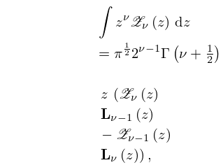
15: 10.43 Integrals

… ►Let

\mathscr{Z}_{\nu}\left(z\right)

be defined as in §10.25(ii). … ►

\int z^{\nu+1}\mathscr{Z}_{\nu}\left(z\right)\,\mathrm{d}z=z^{\nu+1}\mathscr{Z% }_{\nu+1}\left(z\right),

… ►

10.43.2

\int z^{\nu}\mathscr{Z}_{\nu}\left(z\right)\,\mathrm{d}z=\pi^{\frac{1}{2}}2^{% \nu-1}\Gamma\left(\nu+\tfrac{1}{2}\right)z\*\left(\mathscr{Z}_{\nu}\left(z% \right)\mathbf{L}_{\nu-1}\left(z\right)-\mathscr{Z}_{\nu-1}\left(z\right)% \mathbf{L}_{\nu}\left(z\right)\right),

\nu\neq-\tfrac{1}{2}

ⓘ

Symbols:: $\Gamma\left(\NVar{z}\right)$ : gamma function, $\pi$ : the ratio of the circumference of a circle to its diameter, $\,\mathrm{d}\NVar{x}$ : differential of $x$ , $\int$ : integral, $\mathbf{L}_{\NVar{\nu}}\left(\NVar{z}\right)$ : modified Struve function, $\mathscr{Z}_{\NVar{\nu}}\left(\NVar{z}\right)$ : modified cylinder function, $z$ : complex variable and $\nu$ : complex parameter
A&S Ref:: 11.1.8 (Case $\nu=0$ only)
Referenced by:: §10.43(i)
Permalink:: http://dlmf.nist.gov/10.43.E2
Encodings:: pMML, png, TeX
See also:: Annotations for §10.43(i), §10.43 and Ch.10

… ►

\int e^{\pm z}z^{\nu}\mathscr{Z}_{\nu}\left(z\right)\,\mathrm{d}z=\frac{e^{\pm z% }z^{\nu+1}}{2\nu+1}\left(\mathscr{Z}_{\nu}\left(z\right)\mp\mathscr{Z}_{\nu+1}% \left(z\right)\right),

\nu\neq-\tfrac{1}{2}

►

\int e^{\pm z}z^{-\nu}\mathscr{Z}_{\nu}\left(z\right)\,\mathrm{d}z=\frac{e^{% \pm z}z^{-\nu+1}}{1-2\nu}\left(\mathscr{Z}_{\nu}\left(z\right)\mp\mathscr{Z}_{% \nu-1}\left(z\right)\right),

\nu\neq\tfrac{1}{2}

…

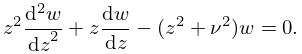
16: 10.25 Definitions

… ►

10.25.1

z^{2}\frac{{\mathrm{d}}^{2}w}{{\mathrm{d}z}^{2}}+z\frac{\mathrm{d}w}{\mathrm{d% }z}-(z^{2}+\nu^{2})w=0.

ⓘ

Symbols:: $\frac{\mathrm{d}\NVar{f}}{\mathrm{d}\NVar{x}}$ : derivative of $f$ with respect to $x$ , $z$ : complex variable and $\nu$ : complex parameter
A&S Ref:: 9.6.1
Referenced by:: §10.25(ii), §10.25(iii), §10.27, §10.45, §10.74(ii)
Permalink:: http://dlmf.nist.gov/10.25.E1
Encodings:: pMML, png, TeX
See also:: Annotations for §10.25(i), §10.25 and Ch.10

… ►In particular, the principal branch of

I_{\nu}\left(z\right)

is defined in a similar way: it corresponds to the principal value of

(\tfrac{1}{2}z)^{\nu}

, is analytic in

\mathbb{C}\setminus(-\infty,0]

, and two-valued and discontinuous on the cut

\operatorname{ph}z=\pm\pi

. … ►as

z\to\infty

|\operatorname{ph}z|\leq\tfrac{3}{2}\pi-\delta

(<\tfrac{3}{2}\pi)

. … ►

Symbol $\mathscr{Z}_{\nu}\left(z\right)$

►Corresponding to the symbol

\mathscr{C}_{\nu}

introduced in §10.2(ii), we sometimes use

\mathscr{Z}_{\nu}\left(z\right)

to denote

I_{\nu}\left(z\right)

e^{\nu\pi i}K_{\nu}\left(z\right)

, or any nontrivial linear combination of these functions, the coefficients in which are independent of

z

and

\nu

. …

17: 22.21 Tables

… ►Curtis (1964b) tabulates

\operatorname{sn}\left(mK/n,k\right)

\operatorname{cn}\left(mK/n,k\right)

\operatorname{dn}\left(mK/n,k\right)

for

n=2(1)15

m=1(1)n-1

, and

q

(not

k

)

=0(.005)0.35

to 20D. ►Lawden (1989, pp. 280–284 and 293–297) tabulates

\operatorname{sn}\left(x,k\right)

\operatorname{cn}\left(x,k\right)

\operatorname{dn}\left(x,k\right)

\mathcal{E}\left(x,k\right)

\mathrm{Z}\left(x|k\right)

to 5D for

k=0.1(.1)0.9

x=0(.1)X

, where

X

ranges from 1. 5 to 2. 2. … ►Zhang and Jin (1996, p. 678) tabulates

\operatorname{sn}\left(Kx,k\right)

\operatorname{cn}\left(Kx,k\right)

\operatorname{dn}\left(Kx,k\right)

for

k=\frac{1}{4},\frac{1}{2}

and

x=0(.1)4

to 7D. …

18: 35.1 Special Notation

… ► ►►►►

$a, b$	complex variables.
…
$\mathbf{Z}$	complex symmetric matrix.
…
$Z_{\kappa}\left(\mathbf{T}\right)$	zonal polynomials.

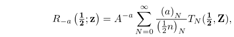
►The main functions treated in this chapter are the multivariate gamma and beta functions, respectively

\Gamma_{m}\left(a\right)

and

\mathrm{B}_{m}\left(a,b\right)

, and the special functions of matrix argument: Bessel (of the first kind)

A_{\nu}\left(\mathbf{T}\right)

and (of the second kind)

B_{\nu}\left(\mathbf{T}\right)

; confluent hypergeometric (of the first kind)

{{}_{1}F_{1}}\left(a;b;\mathbf{T}\right)

\displaystyle{{}_{1}F_{1}}\left({a\atop b};\mathbf{T}\right)

and (of the second kind)

\Psi\left(a;b;\mathbf{T}\right)

; Gaussian hypergeometric

{{}_{2}F_{1}}\left(a_{1},a_{2};b;\mathbf{T}\right)

\displaystyle{{}_{2}F_{1}}\left({a_{1},a_{2}\atop b};\mathbf{T}\right)

; generalized hypergeometric

{{}_{p}F_{q}}\left(a_{1},\dots,a_{p};b_{1},\dots,b_{q};\mathbf{T}\right)

\displaystyle{{}_{p}F_{q}}\left({a_{1},\dots,a_{p}\atop b_{1},\dots,b_{q}};% \mathbf{T}\right)

. ►An alternative notation for the multivariate gamma function is

\Pi_{m}(a)=\Gamma_{m}\left(a+\tfrac{1}{2}(m+1)\right)

(Herz (1955, p. 480)). Related notations for the Bessel functions are

\mathcal{J}_{\nu+\frac{1}{2}(m+1)}(\mathbf{T})=A_{\nu}\left(\mathbf{T}\right)/% A_{\nu}\left(\boldsymbol{{0}}\right)

(Faraut and Korányi (1994, pp. 320–329)),

K_{m}(0,\dots,0,\nu\mathpunct{|}\mathbf{S},\mathbf{T})=\left|\mathbf{T}\right|% ^{\nu}B_{\nu}\left(\mathbf{S}\mathbf{T}\right)

(Terras (1988, pp. 49–64)), and

\mathcal{K}_{\nu}(\mathbf{T})=\left|\mathbf{T}\right|^{\nu}B_{\nu}\left(% \mathbf{S}\mathbf{T}\right)

(Faraut and Korányi (1994, pp. 357–358)).

19: 10.66 Expansions in Series of Bessel Functions

… ►

10.66.1

\operatorname{ber}_{\nu}x+i\operatorname{bei}_{\nu}x=\sum_{k=0}^{\infty}\frac{% e^{(3\nu+k)\pi i/4}x^{k}J_{\nu+k}\left(x\right)}{2^{k/2}k!}=\sum_{k=0}^{\infty% }\frac{e^{(3\nu+3k)\pi i/4}x^{k}I_{\nu+k}\left(x\right)}{2^{k/2}k!}.

ⓘ

Symbols:: $J_{\NVar{\nu}}\left(\NVar{z}\right)$ : Bessel function of the first kind, $\operatorname{bei}_{\NVar{\nu}}\left(\NVar{x}\right)$ : Kelvin function, $\operatorname{ber}_{\NVar{\nu}}\left(\NVar{x}\right)$ : Kelvin function, $\pi$ : the ratio of the circumference of a circle to its diameter, $\mathrm{e}$ : base of natural logarithm, $!$ : factorial (as in $n!$ ), $\mathrm{i}$ : imaginary unit, $I_{\NVar{\nu}}\left(\NVar{z}\right)$ : modified Bessel function of the first kind, $k$ : nonnegative integer, $x$ : real variable and $\nu$ : complex parameter
A&S Ref:: 9.9.32
Referenced by:: §10.66
Permalink:: http://dlmf.nist.gov/10.66.E1
Encodings:: pMML, png, TeX
See also:: Annotations for §10.66 and Ch.10

►

\operatorname{ber}_{n}\left(x\sqrt{2}\right)=\sum_{k=-\infty}^{\infty}(-1)^{n+% k}J_{n+2k}\left(x\right)I_{2k}\left(x\right),

►

\operatorname{bei}_{n}\left(x\sqrt{2}\right)=\sum_{k=-\infty}^{\infty}(-1)^{n+% k}J_{n+2k+1}\left(x\right)I_{2k+1}\left(x\right).

20: 19.36 Methods of Computation

… ►where, in the notation of (19.19.7) with

a=-\frac{1}{2}

and

n=3

, … ►where

n=0,1,2,\dots

, and … ►This method loses significant figures in

\rho

\alpha^{2}

and

k^{2}

are nearly equal unless they are given exact values—as they can be for tables. If

\alpha^{2}=k^{2}

, then the method fails, but the function can be expressed by (19.6.13) in terms of

E\left(\phi,k\right)

, for which Neuman (1969b) uses ascending Landen transformations. … ►The cases

k_{c}^{2}/2\leq p<\infty

and

-\infty <mrow> <mrow> <mo>−</mo> <mi mathvariant=

require different treatment for numerical purposes, and again precautions are needed to avoid cancellations. …