Riemann
(0.001 seconds)
21—30 of 91 matching pages
21: 15.11 Riemann’s Differential Equation
§15.11 Riemann’s Differential Equation
►§15.11(i) Equations with Three Singularities
… ►The complete set of solutions of (15.11.1) is denoted by Riemann’s -symbol: … ►§15.11(ii) Transformation Formulas
… ►for arbitrary and .22: 21.8 Abelian Functions
§21.8 Abelian Functions
… ►For every Abelian function, there is a positive integer , such that the Abelian function can be expressed as a ratio of linear combinations of products with factors of Riemann theta functions with characteristics that share a common period lattice. …23: 21.1 Special Notation
…
►
►
…
►Uppercase boldface letters are real or complex matrices.
►The main functions treated in this chapter are the Riemann theta functions , and the Riemann theta functions with characteristics .
►The function is also commonly used; see, for example, Belokolos et al. (1994, §2.5), Dubrovin (1981), and Fay (1973, Chapter 1).
| positive integers. | |
| … | |
| complex, symmetric matrix with strictly positive definite, i.e., a Riemann matrix. | |
| … | |
| intersection index of and , two cycles lying on a closed surface. if and do not intersect. Otherwise gets an additive contribution from every intersection point. This contribution is if the basis of the tangent vectors of the and cycles (§21.7(i)) at the point of intersection is positively oriented; otherwise it is . | |
| … | |
24: 25.19 Tables
…
►
•
…
►
•
►
•
Fletcher et al. (1962, §22.1) lists many sources for earlier tables of for both real and complex . §22.133 gives sources for numerical values of coefficients in the Riemann–Siegel formula, §22.15 describes tables of values of , and §22.17 lists tables for some Dirichlet -functions for real characters. For tables of dilogarithms, polylogarithms, and Clausen’s integral see §§22.84–22.858.
25: 25.2 Definition and Expansions
§25.2 Definition and Expansions
… ►Elsewhere is defined by analytic continuation. … ►§25.2(ii) Other Infinite Series
… ►§25.2(iii) Representations by the Euler–Maclaurin Formula
… ►§25.2(iv) Infinite Products
…26: 25.16 Mathematical Applications
§25.16 Mathematical Applications
… ►which is related to the Riemann zeta function by … ►The Riemann hypothesis is equivalent to the statement … ►§25.16(ii) Euler Sums
… ►which satisfies the reciprocity law …27: Sidebar 21.SB2: A two-phase solution of the Kadomtsev–Petviashvili equation (21.9.3)
…
►Such a solution is given in terms of a Riemann theta function with two phases.
…
28: 25.5 Integral Representations
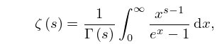
§25.5 Integral Representations
… ►
25.5.1
.
…
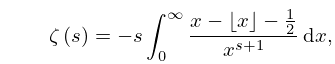
►
25.5.5
.
…
►
25.5.19
.
►
§25.5(iii) Contour Integrals
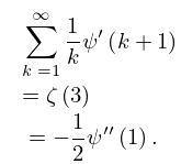
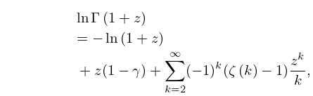
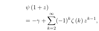
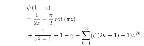
…29: 5.16 Sums
…
►
5.16.2
…
