Mobius inversion formulas

SearchAdvancedHelp

(0.001 seconds)

21—30 of 341 matching pages

21: 4.47 Approximations

§4.47 Approximations

►

§4.47(i) Chebyshev-Series Expansions

►Clenshaw (1962) and Luke (1975, Chapter 3) give 20D coefficients for $\ln$, $\exp$, $\sin$, $\cos$, $\tan$, $\cot$, $\arcsin$, $\arctan$, $\mathrm{arcsinh}$. … ►Hart et al. (1968) give $\ln$, $\exp$, $\sin$, $\cos$, $\tan$, $\cot$, $\arcsin$, $\arccos$, $\arctan$, $\sinh$, $\cosh$, $\tanh$, $\mathrm{arcsinh}$, $\mathrm{arccosh}$. … ►Luke (1975, Chapter 3) supplies real and complex approximations for $\ln$, $\exp$, $\sin$, $\cos$, $\tan$, $\arctan$, $\mathrm{arcsinh}$. …

22: 4.29 Graphics

… ►

§4.29(i) Real Arguments

… ►

►►

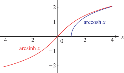
Figure 4.29.2: Principal values of $\mathrm{arcsinh}x$ and $\mathrm{arccosh}x$. … Magnify

… ►

►►

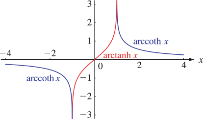
Figure 4.29.4: Principal values of $\mathrm{arctanh}x$ and $\mathrm{arccoth}x$. … Magnify

… ►

§4.29(ii) Complex Arguments

… ►The surfaces for the complex hyperbolic and inverse hyperbolic functions are similar to the surfaces depicted in §4.15(iii) for the trigonometric and inverse trigonometric functions. …

23: 19.11 Addition Theorems

… ►

§19.11(i) General Formulas

… ►

19.11.5 $$\mathrm{\Pi }(\theta ,{\alpha }^2,k)+\mathrm{\Pi }(\varphi ,{\alpha }^2,k)=\mathrm{\Pi }(\psi ,{\alpha }^2,k)-{\alpha }^2{R}_C(\gamma -\delta ,\gamma ),$$

ⓘ

Symbols:

$R_C(x,y)$: Carlson’s combination of inverse circular and inverse hyperbolic functions, $\mathrm{\Pi }(\varphi ,{\alpha }^2,k)$: Legendre’s incomplete elliptic integral of the third kind, $\varphi$: real or complex argument, $k$: real or complex modulus, ${\alpha }^2$: real or complex parameter, $\theta$: amplitude, $\psi$: angle, $\gamma$ and $\delta$

Referenced by:

§19.11(i), §19.11(i), Erratum (V1.0.24) for Subsection 19.11(i)

Permalink:

http://dlmf.nist.gov/19.11.E5

Encodings:

pMML, png, TeX

See also:

Annotations for §19.11(i), §19.11 and Ch.19

… ►

19.11.6_5 $$R_C(\gamma -\delta ,\gamma )=\frac{-1}{\sqrt{\delta }}\arctan \left(\frac{\sqrt{\delta }\sin \theta \sin \varphi \sin \psi }{{\alpha }^2-1-{\alpha }^2\cos \theta \cos \varphi \cos \psi }\right).$$

ⓘ

Symbols:

$R_C(x,y)$: Carlson’s combination of inverse circular and inverse hyperbolic functions, $\cos z$: cosine function, $\arctan z$: arctangent function, $\sin z$: sine function, $\varphi$: real or complex argument, ${\alpha }^2$: real or complex parameter, $\theta$: amplitude, $\psi$: angle, $\gamma$ and $\delta$

Referenced by:

§19.11(i), Erratum (V1.0.28) for Equations (15.2.3_5), (19.11.6_5)

Permalink:

http://dlmf.nist.gov/19.11.E6_5

Encodings:

pMML, png, TeX

Clarification (effective with 1.0.28):

This equation was given a number.

See also:

Annotations for §19.11(i), §19.11 and Ch.19

… ►

§19.11(iii) Duplication Formulas

… ►

19.11.16 $$\mathrm{\Pi }(\psi ,{\alpha }^2,k)=2\mathrm{\Pi }(\theta ,{\alpha }^2,k)+{\alpha }^2{R}_C(\gamma -\delta ,\gamma ),$$

ⓘ

Symbols:

$R_C(x,y)$: Carlson’s combination of inverse circular and inverse hyperbolic functions, $\mathrm{\Pi }(\varphi ,{\alpha }^2,k)$: Legendre’s incomplete elliptic integral of the third kind, $k$: real or complex modulus, ${\alpha }^2$: real or complex parameter, $\theta$: amplitude, $\delta$ , $\psi$: angle and $\gamma$

Permalink:

http://dlmf.nist.gov/19.11.E16

Encodings:

pMML, png, TeX

See also:

Annotations for §19.11(iii), §19.11 and Ch.19

…

24: 4.1 Special Notation

… ►The main purpose of the present chapter is to extend these definitions and properties to complex arguments $z$. ►The main functions treated in this chapter are the logarithm $\ln z$, $\mathrm{Ln}z$; the exponential $\exp z$, ${\mathrm{e}}^z$; the circular trigonometric (or just trigonometric) functions $\sin z$, $\cos z$, $\tan z$, $\csc z$, $\sec z$, $\cot z$; the inverse trigonometric functions $\arcsin z$, $\mathrm{Arcsin}z$, etc. ; the hyperbolic trigonometric (or just hyperbolic) functions $\sinh z$, $\cosh z$, $\tanh z$, $\mathrm{csch}z$, $\mathrm{sech}z$, $\coth z$; the inverse hyperbolic functions $\mathrm{arcsinh}z$, $\mathrm{Arcsinh}z$, etc. ►Sometimes in the literature the meanings of $\ln$ and $\mathrm{Ln}$ are interchanged; similarly for $\arcsin z$ and $\mathrm{Arcsin}z$, etc. …${\sin }^{-1}z$ for $\arcsin z$ and ${\mathrm{Sin}}^{-1}z$ for $\mathrm{Arcsin}z$.

25: 20.11 Generalizations and Analogs

… ►If both $m,n$ are positive, then $G(m,n)$ allows inversion of its arguments as a modular transformation (compare (23.15.3) and (23.15.4)): … ►This is Jacobi’s inversion problem of §20.9(ii). … ►Each provides an extension of Jacobi’s inversion problem. … ►Such sets of twelve equations include derivatives, differential equations, bisection relations, duplication relations, addition formulas (including new ones for theta functions), and pseudo-addition formulas. …

26: 19.26 Addition Theorems

… ►

§19.26(i) General Formulas

… ►

19.26.11 $$R_C(x+\lambda ,y+\lambda )+R_C(x+\mu ,y+\mu )=R_C(x,y),$$

ⓘ

Symbols:

$R_C(x,y)$: Carlson’s combination of inverse circular and inverse hyperbolic functions, $\lambda$: positive, $x$: positive, $y$: positive and $\mu >0$: parameter

Referenced by:

§19.26(i)

Permalink:

http://dlmf.nist.gov/19.26.E11

Encodings:

pMML, png, TeX

See also:

Annotations for §19.26(i), §19.26 and Ch.19

… ►

§19.26(iii) Duplication Formulas

… ►The equations inverse to $z+\lambda =(\sqrt{z}+\sqrt{x})(\sqrt{z}+\sqrt{y})$ and the two other equations obtained by permuting $x,y,z$ (see (19.26.19)) are … ►

19.26.25 $$R_C(x,y)=2R_C(x+\lambda ,y+\lambda ),$$ $\lambda =y+2\sqrt{x}\sqrt{y}$.

ⓘ

Symbols:

$R_C(x,y)$: Carlson’s combination of inverse circular and inverse hyperbolic functions, $\lambda$: positive, $x$: positive and $y$: positive

Referenced by:

§19.26(iii)

Permalink:

http://dlmf.nist.gov/19.26.E25

Encodings:

pMML, png, TeX

See also:

Annotations for §19.26(iii), §19.26 and Ch.19

…

27: 22.21 Tables

… ►Spenceley and Spenceley (1947) tabulates $\mathrm{sn}(Kx,k)$, $\mathrm{cn}(Kx,k)$, $\mathrm{dn}(Kx,k)$, $\mathrm{am}(Kx,k)$, $ℰ(Kx,k)$ for $\arcsin k=1^{\circ }(1^{\circ }){89}^{\circ }$ and $x=0\left(\frac{1}{90}\right)1$ to 12D, or 12 decimals of a radian in the case of $\mathrm{am}(Kx,k)$. … ►Tables of theta functions (§20.15) can also be used to compute the twelve Jacobian elliptic functions by application of the quotient formulas given in §22.2.

28: 6.14 Integrals

… ►

6.14.3 $${\int }_0^{\mathrm{\infty }}{\mathrm{e}}^{-at}\mathrm{si}\left(t\right)dt=-\frac{1}{a}\arctan a,$$ $\mathrm{\Re }a>0$.

ⓘ

Symbols:

$dx$: differential of $x$ , $\mathrm{e}$: base of natural logarithm, $\int$: integral, $\arctan z$: arctangent function, $\mathrm{\Re }$: real part and $\mathrm{si}\left(z\right)$: sine integral

A&S Ref:

5.2.29

Permalink:

http://dlmf.nist.gov/6.14.E3

Encodings:

pMML, png, TeX

See also:

Annotations for §6.14(i), §6.14 and Ch.6

…

29: 6.18 Methods of Computation

… ►For large $x$ and $\left|z\right|$, expansions in inverse factorial series (§6.10(i)) or asymptotic expansions (§6.12) are available. …Also, other ranges of $\mathrm{ph}z$ can be covered by use of the continuation formulas of §6.4. … ►For example, the Gauss–Laguerre formula (§3.5(v)) can be applied to (6.2.2); see Todd (1954) and Tseng and Lee (1998). For an application of the Gauss–Legendre formula (§3.5(v)) see Tooper and Mark (1968). …

30: Bibliography I

… ►

Centre for Experimental and Constructive Mathematics, Simon Fraser University, Canada.

ⓘ

Notes:

From a decimal approximation, find the most likely exact value.

External Links:

Inverse Symbolic Calculator

Referenced by:

3rd item.

Encodings:

BibTeX

… ►

The method of isomonodromic deformations and relation formulas for the second Painlevé transcendent. Izv. Akad. Nauk SSSR Ser. Mat. 51 (4), pp. 878–892, 912 (Russian).

ⓘ

Notes:

In Russian. English translation: Math. USSR-Izv. 31(1988), no. 1, pp. 193–207

External Links:

ISSN 0373-2436, Document, MathReview (Alexander A. Pankov), ZentralBlatt

Referenced by:

§32.11(iii).

Encodings:

BibTeX

… ►

Connection formulae for the fourth Painlevé transcendent; Clarkson-McLeod solution. J. Phys. A 31 (17), pp. 4073–4113.

ⓘ

External Links:

ISSN 0305-4470, Document, MathReview (Yoshitsugu Takei), ZentralBlatt

Referenced by:

§32.11(v).

Encodings:

BibTeX

…