Minkowski’s

SearchAdvancedHelp

(0.002 seconds)

21—30 of 601 matching pages

21: 20.8 Watson’s Expansions

§20.8 Watson’s Expansions

…

22: 31.17 Physical Applications

§31.17 Physical Applications

►

§31.17(i) Addition of Three Quantum Spins

… ►We use vector notation $[𝐬,𝐭,𝐮]$ (respective scalar $(s,t,u)$) for any one of the three spin operators (respective spin values). ►Consider the following spectral problem on the sphere $S_2$: ${𝐱}^2=x_s^2+x_t^2+x_u^2=R^2$. … ►For applications of Heun’s equation and functions in astrophysics see Debosscher (1998) where different spectral problems for Heun’s equation are also considered. …

23: 31.6 Path-Multiplicative Solutions

§31.6 Path-Multiplicative Solutions

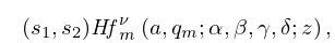
►A further extension of the notation (31.4.1) and (31.4.3) is given by ►

31.6.1 $$(s_1,s_2){\mathrm{𝐻𝑓}}_m^{\nu }(a,q_m;\alpha ,\beta ,\gamma ,\delta ;z),$$ $m=0,1,2,\mathrm{\dots }$,

ⓘ

Symbols:

$(s_1,s_2){\mathrm{𝐻𝑓}}_m(a,q_m;\alpha ,\beta ,\gamma ,\delta ;z)$: Heun functions, $z$: complex variable, $\gamma$: real or complex parameter, $\delta$: real or complex parameter, $\nu$: real or complex parameter, $m$: nonnegative integer, $a$: complex parameter, $q$: real or complex parameter, $\alpha$: real or complex parameter, $\beta$: real or complex parameter and $s_j$: parameters

Permalink:

http://dlmf.nist.gov/31.6.E1

Encodings:

pMML, png, TeX

See also:

Annotations for §31.6 and Ch.31

►with $(s_1,s_2)\in \{0,1,a\}$, but with another set of $\{q_m\}$. This denotes a set of solutions of (31.2.1) with the property that if we pass around a simple closed contour in the $z$-plane that encircles $s_1$ and $s_2$ once in the positive sense, but not the remaining finite singularity, then the solution is multiplied by a constant factor ${\mathrm{e}}^{2\nu \pi \mathrm{i}}$. …

24: 29.14 Orthogonality

… ►

29.14.2 $$⟨g,h⟩={\int }_0^K{\int }_0^{K^{\prime }}w(s,t)g(s,t)h(s,t)dtds,$$

ⓘ

Symbols:

$K^{\prime }\left(k\right)$: Legendre’s complementary complete elliptic integral of the first kind, $K\left(k\right)$: Legendre’s complete elliptic integral of the first kind, $dx$: differential of $x$ , $\int$: integral, $k$: real parameter and $w(s,t)$: function

Referenced by:

§29.14

Permalink:

http://dlmf.nist.gov/29.14.E2

Encodings:

pMML, png, TeX

See also:

Annotations for §29.14 and Ch.29

►where ►

29.14.3 $$w(s,t)={\mathrm{sn}}^2(K+\mathrm{i}t,k)-{\mathrm{sn}}^2(s,k).$$

ⓘ

Symbols:

$\mathrm{sn}(z,k)$: Jacobian elliptic function, $K\left(k\right)$: Legendre’s complete elliptic integral of the first kind, $\mathrm{i}$: imaginary unit, $k$: real parameter and $w(s,t)$: function

Referenced by:

§29.14

Permalink:

http://dlmf.nist.gov/29.14.E3

Encodings:

pMML, png, TeX

See also:

Annotations for §29.14 and Ch.29

… ►

29.14.11 $$⟨g,h⟩={\int }_0^{4K}{\int }_0^{2K^{\prime }}w(s,t)g(s,t)h(s,t)dtds,$$

ⓘ

Symbols:

$K^{\prime }\left(k\right)$: Legendre’s complementary complete elliptic integral of the first kind, $K\left(k\right)$: Legendre’s complete elliptic integral of the first kind, $dx$: differential of $x$ , $\int$: integral, $k$: real parameter and $w(s,t)$: function

Permalink:

http://dlmf.nist.gov/29.14.E11

Encodings:

pMML, png, TeX

See also:

Annotations for §29.14 and Ch.29

►with $w(s,t)$ given by (29.14.3).

25: 28.17 Stability as $x\to \pm \mathrm{\infty }$

§28.17 Stability as $x\to \pm \mathrm{\infty }$

… ► ►

►►

Figure 28.17.1: Stability chart for eigenvalues of Mathieu’s equation (28.2.1). Magnify

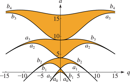26: 25.2 Definition and Expansions

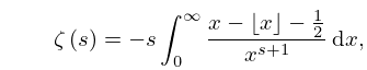
… ►When $\mathrm{\Re }s>1$, …Elsewhere $\zeta \left(s\right)$ is defined by analytic continuation. It is a meromorphic function whose only singularity in $ℂ$ is a simple pole at $s=1$, with residue 1. … ►This includes, for example, $1/\zeta \left(s\right)$. … ►product over zeros $\rho$ of $\zeta$ with $\mathrm{\Re }\rho >0$ (see §25.10(i)); $\gamma$ is Euler’s constant (§5.2(ii)).

27: 25.5 Integral Representations

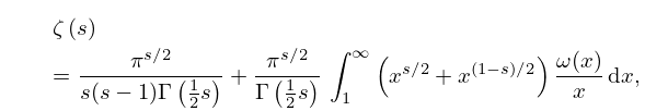
… ►Throughout this subsection $s\ne 1$. … ►

25.5.5 $$\zeta \left(s\right)=-s{\int }_0^{\mathrm{\infty }}\frac{x-\lfloor x\rfloor -\frac{1}{2}}{x^{s+1}}dx,$$ .

ⓘ

Symbols:

$\zeta \left(s\right)$: Riemann zeta function, $dx$: differential of $x$ , $\lfloor x\rfloor$: floor of $x$ , $\int$: integral, $\mathrm{\Re }$: real part, $x$: real variable and $s$: complex variable

Keywords:

improper integral, integral representation

Source:

Titchmarsh (1986b, (2.1.6), p. 15)

Permalink:

http://dlmf.nist.gov/25.5.E5

Encodings:

pMML, png, TeX

See also:

Annotations for §25.5(i), §25.5 and Ch.25

… ►

25.5.13 $$\zeta \left(s\right)=\frac{{\pi }^{s/2}}{s(s-1)\mathrm{\Gamma }\left(\frac{1}{2}s\right)}+\frac{{\pi }^{s/2}}{\mathrm{\Gamma }\left(\frac{1}{2}s\right)}{\int }_1^{\mathrm{\infty }}\left(x^{s/2}+x^{(1-s)/2}\right)\frac{\omega (x)}{x}dx,$$ $s\ne 1$,

ⓘ

Symbols:

$\mathrm{\Gamma }\left(z\right)$: gamma function, $\zeta \left(s\right)$: Riemann zeta function, $\pi$: the ratio of the circumference of a circle to its diameter, $dx$: differential of $x$ , $\int$: integral, $x$: real variable and $s$: complex variable

Keywords:

improper integral, integral representation

Source:

Titchmarsh (1986b, p. 22)

Permalink:

http://dlmf.nist.gov/25.5.E13

Encodings:

pMML, png, TeX

See also:

Annotations for §25.5(ii), §25.5 and Ch.25

… ►In (25.5.15)–(25.5.19), , $\psi \left(x\right)$ is the digamma function, and $\gamma$ is Euler’s constant (§5.2). (25.5.16) is also valid for , $s\ne 1$. …

28: 25.15 Dirichlet $L$-functions

… ►If $\chi \ne {\chi }_1$, then $L(s,\chi )$ is an entire function of $s$. …This implies that $L(s,\chi )\ne 0$ if $\mathrm{\Re }s>1$. … ►Since $L(s,\chi )\ne 0$ if $\mathrm{\Re }s>1$, (25.15.5) shows that for a primitive character $\chi$ the only zeros of $L(s,\chi )$ for (the so-called trivial zeros) are as follows: … ►This result plays an important role in the proof of Dirichlet’s theorem on primes in arithmetic progressions (§27.11). Related results are: …

29: 26.1 Special Notation

… ► ►►►►

$\left(\genfrac{}{}{0.0pt}{}{m}{n}\right)$	binomial coefficient.
…
$s(n,k)$	Stirling numbers of the first kind.
$S(n,k)$	Stirling numbers of the second kind.

… ►Other notations for $s(n,k)$, the Stirling numbers of the first kind, include $S_n^{(k)}$ (Abramowitz and Stegun (1964, Chapter 24), Fort (1948)), $S_n^k$ (Jordan (1939), Moser and Wyman (1958a)), $\left(\genfrac{}{}{0.0pt}{}{n-1}{k-1}\right)B_{n-k}^{(n)}$ (Milne-Thomson (1933)), ${(-1)}^{n-k}{S}_1(n-1,n-k)$ (Carlitz (1960), Gould (1960)), ${(-1)}^{n-k}\left[\genfrac{}{}{0pt}{}{n}{k}\right]$ (Knuth (1992), Graham et al. (1994), Rosen et al. (2000)). ►Other notations for $S(n,k)$, the Stirling numbers of the second kind, include ${𝒮}_n^{(k)}$ (Fort (1948)), ${𝔖}_n^k$ (Jordan (1939)), ${\sigma }_n^k$ (Moser and Wyman (1958b)), $\left(\genfrac{}{}{0.0pt}{}{n}{k}\right)B_{n-k}^{(-k)}$ (Milne-Thomson (1933)), $S_2(k,n-k)$ (Carlitz (1960), Gould (1960)), $\left\{\genfrac{}{}{0pt}{}{n}{k}\right\}$ (Knuth (1992), Graham et al. (1994), Rosen et al. (2000)), and also an unconventional symbol in Abramowitz and Stegun (1964, Chapter 24).

30: 25.19 Tables

… ►

Abramowitz and Stegun (1964) tabulates: $\zeta \left(n\right)$, $n=2,3,4,\mathrm{\dots }$, 20D (p. 811); ${\mathrm{Li}}_2\left(1-x\right)$, $x=0(.01)0.5$, 9D (p. 1005); $f(\theta )$, $\theta ={15}^{\circ }(1^{\circ }){30}^{\circ }(2^{\circ }){90}^{\circ }(5^{\circ }){180}^{\circ }$, $f(\theta )+\theta \ln \theta$, $\theta =0(1^{\circ }){15}^{\circ }$, 6D (p. 1006). Here $f(\theta )$ denotes Clausen’s integral, given by the right-hand side of (25.12.9).

… ►

Cloutman (1989) tabulates $\mathrm{\Gamma }\left(s+1\right)F_s(x)$, where $F_s(x)$ is the Fermi–Dirac integral (25.12.14), for $s=-\frac{1}{2},\frac{1}{2},\frac{3}{2},\frac{5}{2}$, $x=-5(.05)25$, to 12S.

►

Fletcher et al. (1962, §22.1) lists many sources for earlier tables of $\zeta \left(s\right)$ for both real and complex $s$. §22.133 gives sources for numerical values of coefficients in the Riemann–Siegel formula, §22.15 describes tables of values of $\zeta (s,a)$, and §22.17 lists tables for some Dirichlet $L$-functions for real characters. For tables of dilogarithms, polylogarithms, and Clausen’s integral see §§22.84–22.858.