Legendre polynomials

SearchAdvancedHelp

(0.007 seconds)

21—30 of 71 matching pages

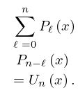
21: 18.18 Sums

… ►

Legendre

… ►

18.18.3 $$a_n=\left(n+\frac{1}{2}\right){\int }_{-1}^{1}f(x)P_n\left(x\right)dx.$$

ⓘ

Symbols:

$P_n\left(x\right)$: Legendre polynomial, $dx$: differential of $x$ , $\int$: integral, $n$: nonnegative integer, $f(z)$: analytic function, $a_n$ and $x$: real variable

Permalink:

http://dlmf.nist.gov/18.18.E3

Encodings:

pMML, png, TeX

See also:

Annotations for §18.18(i), §18.18(i), §18.18 and Ch.18

… ►

Legendre

… ►

Legendre and Chebyshev

►

18.18.36 $$\sum _{\mathrm{\ell }=0}^n{P}_{\mathrm{\ell }}\left(x\right)P_{n-\mathrm{\ell }}\left(x\right)=U_n\left(x\right).$$

ⓘ

Symbols:

$U_n\left(x\right)$: Chebyshev polynomial of the second kind, $P_n\left(x\right)$: Legendre polynomial, $\mathrm{\ell }$: nonnegative integer, $n$: nonnegative integer and $x$: real variable

Referenced by:

§18.18(viii)

Permalink:

http://dlmf.nist.gov/18.18.E36

Encodings:

pMML, png, TeX

See also:

Annotations for §18.18(viii), §18.18(viii), §18.18 and Ch.18

…

22: 18.15 Asymptotic Approximations

… ►

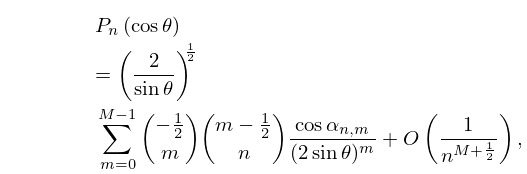
§18.15(iii) Legendre

… ►

18.15.12 $$P_n\left(\cos \theta \right)={\left(\frac{2}{\sin \theta }\right)}^{\frac{1}{2}}\sum _{m=0}^{M-1}\left(\genfrac{}{}{0.0pt}{}{-\frac{1}{2}}{m}\right)\left(\genfrac{}{}{0.0pt}{}{m-\frac{1}{2}}{n}\right)\frac{\cos {\alpha }_{n,m}}{{(2\sin \theta )}^m}+O\left(\frac{1}{n^{M+\frac{1}{2}}}\right),$$

ⓘ

Symbols:

$O\left(x\right)$: order not exceeding, $P_n\left(x\right)$: Legendre polynomial, $\left(\genfrac{}{}{0.0pt}{}{m}{n}\right)$: binomial coefficient, $\cos z$: cosine function, $\sin z$: sine function, $m$: nonnegative integer, $n$: nonnegative integer and ${\alpha }_{n,m}$

Referenced by:

§18.15(iii)

Permalink:

http://dlmf.nist.gov/18.15.E12

Encodings:

pMML, png, TeX

See also:

Annotations for §18.15(iii), §18.15 and Ch.18

… ►Also, when , the right-hand side of (18.15.12) with $M=\mathrm{\infty }$ converges; paradoxically, however, the sum is $2P_n\left(\cos \theta \right)$ and not $P_n\left(\cos \theta \right)$ as stated erroneously in Szegő (1975, §8.4(3)). … ►For asymptotic expansions of $P_n\left(\cos \theta \right)$ and $P_n\left(\cosh \xi \right)$ that are uniformly valid when $0\le \theta \le \pi -\delta$ and see §14.15(iii) with $\mu =0$ and $\nu =n$. …

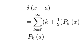
23: 1.17 Integral and Series Representations of the Dirac Delta

… ►

Legendre Polynomials (§§14.7(i) and 18.3)

►

1.17.22 $$\delta \left(x-a\right)=\sum _{k=0}^{\mathrm{\infty }}(k+\frac{1}{2})P_k\left(x\right)P_k\left(a\right).$$

ⓘ

Symbols:

$\delta \left(x-a\right)$: Dirac delta (or Dirac delta function), $P_n\left(x\right)$: Legendre polynomial and $k$: integer

Referenced by:

§1.17(iii), §1.17(iv), §14.18(iii)

Permalink:

http://dlmf.nist.gov/1.17.E22

Encodings:

pMML, png, TeX

See also:

Annotations for §1.17(iii), §1.17(iii), §1.17 and Ch.1

…

24: 2.10 Sums and Sequences

… ►

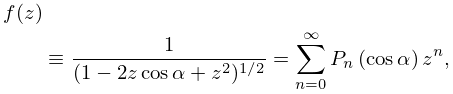
Example

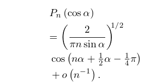
►Let $\alpha$ be a constant in $(0,2\pi )$ and $P_n$ denote the Legendre polynomial of degree $n$. … ►

2.10.33 $$f(z)\equiv \frac{1}{{(1-2z\cos \alpha +z^2)}^{1/2}}=\sum _{n=0}^{\mathrm{\infty }}{P}_n\left(\cos \alpha \right)z^n,$$ .

ⓘ

Symbols:

$P_n\left(x\right)$: Legendre polynomial, $\cos z$: cosine function, $\equiv$: equals by definition and $f(x)$: analytic function

Permalink:

http://dlmf.nist.gov/2.10.E33

Encodings:

pMML, png, TeX

See also:

Annotations for §2.10(iv), §2.10(iv), §2.10 and Ch.2

… ►

2.10.36 $$P_n\left(\cos \alpha \right)={\left(\frac{2}{\pi n\sin \alpha }\right)}^{1/2}\cos \left(n\alpha +\frac{1}{2}\alpha -\frac{1}{4}\pi \right)+o\left(n^{-1}\right).$$

ⓘ

Symbols:

$P_n\left(x\right)$: Legendre polynomial, $\pi$: the ratio of the circumference of a circle to its diameter, $\cos z$: cosine function, $o\left(x\right)$: order less than and $\sin z$: sine function

Permalink:

http://dlmf.nist.gov/2.10.E36

Encodings:

pMML, png, TeX

See also:

Annotations for §2.10(iv), §2.10(iv), §2.10 and Ch.2

…

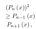
25: 18.14 Inequalities

… ►

Legendre

►

18.14.10 $${(P_n\left(x\right))}^2\ge P_{n-1}\left(x\right)P_{n+1}\left(x\right),$$ $-1\le x\le 1$.

ⓘ

Symbols:

$P_n\left(x\right)$: Legendre polynomial, $n$: nonnegative integer and $x$: real variable

Referenced by:

§18.14(ii)

Permalink:

http://dlmf.nist.gov/18.14.E10

Encodings:

pMML, png, TeX

See also:

Annotations for §18.14(ii), §18.14(ii), §18.14 and Ch.18

…

26: 3.5 Quadrature

… ►The $p_n(x)$ are the monic Legendre polynomials, that is, the polynomials $P_n\left(x\right)$ (§18.3) scaled so that the coefficient of the highest power of $x$ in their explicit forms is unity. … ►

Table 3.5.2: Nodes and weights for the 10-point Gauss–Legendre formula.

► ►►

$\pm x_k$	$w_k$
…

►

►

Table 3.5.3: Nodes and weights for the 20-point Gauss–Legendre formula.

► ►►

$\pm x_k$	$w_k$
…

►

►

Table 3.5.4: Nodes and weights for the 40-point Gauss–Legendre formula.

► ►►

$\pm x_k$	$w_k$
…

►

►

Table 3.5.5: Nodes and weights for the 80-point Gauss–Legendre formula.

► ►►

$\pm x_k$	$w_k$
…

►

…

27: 14.31 Other Applications

… ►Many additional physical applications of Legendre polynomials and associated Legendre functions include solution of the Helmholtz equation, as well as the Laplace equation, in spherical coordinates (Temme (1996b)), quantum mechanics (Edmonds (1974)), and high-frequency scattering by a sphere (Nussenzveig (1965)). …

28: 15.9 Relations to Other Functions

… ►

Legendre

►

15.9.7 $$P_n\left(x\right)=F(\genfrac{}{}{0pt}{}{-n,n+1}{1};\frac{1-x}{2}).$$

ⓘ

Symbols:

$F(a,b;c;z)$ or $F(\genfrac{}{}{0pt}{}{a,b}{c};z)$: $={}_2{}^{}F_1^{}(a,b;c;z)$ Gauss’ hypergeometric function, $P_n\left(x\right)$: Legendre polynomial, $x$: real variable and $n$: integer

Permalink:

http://dlmf.nist.gov/15.9.E7

Encodings:

pMML, png, TeX

See also:

Annotations for §15.9(i), §15.9(i), §15.9 and Ch.15

…

29: 18.16 Zeros

… ►

§18.16(iii) Ultraspherical, Legendre and Chebyshev

►For ultraspherical and Legendre polynomials, set $\alpha =\beta$ and $\alpha =\beta =0$, respectively, in the results given in §18.16(ii). …

30: 29.14 Orthogonality

… ►

29.14.4 $${\mathrm{𝑠𝐸}}_{2n+1}^m(s,k^2){\mathrm{𝑠𝐸}}_{2n+1}^m(K+\mathrm{i}t,k^2),$$

ⓘ

Symbols:

${\mathrm{𝑠𝐸}}_{2n+1}^m(z,k^2)$: Lamé polynomial, $K\left(k\right)$: Legendre’s complete elliptic integral of the first kind, $\mathrm{i}$: imaginary unit, $m$: nonnegative integer, $n$: nonnegative integer and $k$: real parameter

Referenced by:

§29.14

Permalink:

http://dlmf.nist.gov/29.14.E4

Encodings:

pMML, png, TeX

See also:

Annotations for §29.14 and Ch.29

►

29.14.5 $${\mathrm{𝑐𝐸}}_{2n+1}^m(s,k^2){\mathrm{𝑐𝐸}}_{2n+1}^m(K+\mathrm{i}t,k^2),$$

ⓘ

Symbols:

${\mathrm{𝑐𝐸}}_{2n+1}^m(z,k^2)$: Lamé polynomial, $K\left(k\right)$: Legendre’s complete elliptic integral of the first kind, $\mathrm{i}$: imaginary unit, $m$: nonnegative integer, $n$: nonnegative integer and $k$: real parameter

Permalink:

http://dlmf.nist.gov/29.14.E5

Encodings:

pMML, png, TeX

See also:

Annotations for §29.14 and Ch.29

►

29.14.6 $${\mathrm{𝑑𝐸}}_{2n+1}^m(s,k^2){\mathrm{𝑑𝐸}}_{2n+1}^m(K+\mathrm{i}t,k^2),$$

ⓘ

Symbols:

${\mathrm{𝑑𝐸}}_{2n+1}^m(z,k^2)$: Lamé polynomial, $K\left(k\right)$: Legendre’s complete elliptic integral of the first kind, $\mathrm{i}$: imaginary unit, $m$: nonnegative integer, $n$: nonnegative integer and $k$: real parameter

Permalink:

http://dlmf.nist.gov/29.14.E6

Encodings:

pMML, png, TeX

See also:

Annotations for §29.14 and Ch.29

►

29.14.7 $${\mathrm{𝑠𝑐𝐸}}_{2n+2}^m(s,k^2){\mathrm{𝑠𝑐𝐸}}_{2n+2}^m(K+\mathrm{i}t,k^2),$$

ⓘ

Symbols:

${\mathrm{𝑠𝑐𝐸}}_{2n+2}^m(z,k^2)$: Lamé polynomial, $K\left(k\right)$: Legendre’s complete elliptic integral of the first kind, $\mathrm{i}$: imaginary unit, $m$: nonnegative integer, $n$: nonnegative integer and $k$: real parameter

Permalink:

http://dlmf.nist.gov/29.14.E7

Encodings:

pMML, png, TeX

See also:

Annotations for §29.14 and Ch.29

►

29.14.8 $${\mathrm{𝑠𝑑𝐸}}_{2n+2}^m(s,k^2){\mathrm{𝑠𝑑𝐸}}_{2n+2}^m(K+\mathrm{i}t,k^2),$$

ⓘ

Symbols:

${\mathrm{𝑠𝑑𝐸}}_{2n+2}^m(z,k^2)$: Lamé polynomial, $K\left(k\right)$: Legendre’s complete elliptic integral of the first kind, $\mathrm{i}$: imaginary unit, $m$: nonnegative integer, $n$: nonnegative integer and $k$: real parameter

Permalink:

http://dlmf.nist.gov/29.14.E8

Encodings:

pMML, png, TeX

See also:

Annotations for §29.14 and Ch.29

…