DLMF: Untitled Document

§25.15 Dirichlet $L$ -functions

►

§25.15(i) Definitions and Basic Properties

►The notation

L\left(s,\chi\right)

was introduced by Dirichlet (1837) for the meromorphic continuation of the function defined by the series … … ►

§25.15(ii) Zeros

…

… ►

§3.5(i) Trapezoidal Rules

… ►The composite trapezoidal rule is … ►

§3.5(ii) Simpson’s Rule

… ►

§3.5(iv) Interpolatory Quadrature Rules

… ► …

… ►

Chain Rule

… ►

L’Hôpital’s Rule

…

… ►With

\mathbf{y}=[y_{1},y_{2},\dots,y_{n}]^{\rm T}

the process of solution can then be regarded as first solving the equation

\mathbf{L}\mathbf{y}=\mathbf{b}

for

\mathbf{y}

(forward elimination), followed by the solution of

\mathbf{U}\mathbf{x}=\mathbf{y}

for

\mathbf{x}

(back substitution). … ►Because of rounding errors, the residual vector

\mathbf{r}=\mathbf{b}-\mathbf{A}\mathbf{x}

is nonzero as a rule. … ►

3.2.8

\mathbf{L}=\begin{bmatrix}1&0&&&0\\ \ell_{2}&1&0&&\\ &\ddots&\ddots&\ddots&\\ &&\ell_{n-1}&1&0\\ 0&&&\ell_{n}&1\end{bmatrix},

ⓘ

Defines:: $\ell_{jk}$ : elements of $\mathbf{L}$ (locally)
Permalink:: http://dlmf.nist.gov/3.2.E8
Encodings:: pMML, png, TeX
See also:: Annotations for §3.2(ii), §3.2 and Ch.3

… ►In the case that the orthogonality condition is replaced by

\mathbf{S}

-orthogonality, that is,

\mathbf{v}_{j}^{\rm T}\mathbf{S}\mathbf{v}_{k}=\delta_{j,k}

,

j,k=1,2,\ldots,n

, for some positive definite matrix

\mathbf{S}

with Cholesky decomposition

\mathbf{S}=\mathbf{L}^{\rm T}\mathbf{L}

, then the details change as follows. … ►

\mathbf{v}_{j+1}=\ifrac{\mathbf{L}^{-1}\left(\mathbf{L}^{-1}\right)^{\rm T}% \mathbf{u}}{\beta_{j+1}},

…

… ►

34.5.11

{(2j_{1}+1)\left((J_{3}+J_{2}-J_{1})(L_{3}+L_{2}-J_{1})-2(J_{3}L_{3}+J_{2}L_{2% }-J_{1}L_{1})\right)\begin{Bmatrix}j_{1}&j_{2}&j_{3}\\ l_{1}&l_{2}&l_{3}\end{Bmatrix}}\\ =j_{1}E(j_{1}+1)\begin{Bmatrix}j_{1}+1&j_{2}&j_{3}\\ l_{1}&l_{2}&l_{3}\end{Bmatrix}+(j_{1}+1)E(j_{1})\begin{Bmatrix}j_{1}-1&j_{2}&j% _{3}\\ l_{1}&l_{2}&l_{3}\end{Bmatrix},

ⓘ

Symbols:: $\begin{Bmatrix}\NVar{j_{1}}&\NVar{j_{2}}&\NVar{j_{3}}\\ \NVar{l_{1}}&\NVar{l_{2}}&\NVar{l_{3}}\end{Bmatrix}$ : $\mathit{6j}$ symbol, $j,j_{r}$ : non-negative integers or non-negative integers plus one half., $l,l_{r}$ : non-negative integers or non-negative integers plus one half., $J_{r}$ , $L_{r}$ and $E(j)$
Permalink:: http://dlmf.nist.gov/34.5.E11
Encodings:: pMML, png, TeX
See also:: Annotations for §34.5(iii), §34.5 and Ch.34

… ►

L_{r}=l_{r}(l_{r}+1),

… ►Equations (34.5.15) and (34.5.16) are the sum rules. They constitute addition theorems for the

\mathit{6j}

symbol. …

… ►

See accompanying text — Figure 18.4.5: Laguerre polynomials $L_{n}\left(x\right)$ , $n=1,2,3,4,5$ . Magnify

►

… ►

►

… ►

23.10.10

\sigma\left(2z\right)=-\wp'\left(z\right){\sigma}^{4}\left(z\right).

ⓘ

Symbols:: $\wp\left(\NVar{z}\right)$ (= $\wp\left(z|\mathbb{L}\right)$ = $\wp\left(z;g_{2},g_{3}\right)$ ): Weierstrass $\wp$ -function, $\sigma\left(\NVar{z}\right)$ (= $\sigma\left(z|\mathbb{L}\right)$ = $\sigma\left(z;g_{2},g_{3}\right)$ ): Weierstrass sigma function, $\mathbb{L}$ : lattice and $z$ : complex
A&S Ref:: 18.4.8
Referenced by:: §23.10(ii)
Permalink:: http://dlmf.nist.gov/23.10.E10
Encodings:: pMML, png, TeX
See also:: Annotations for §23.10(ii), §23.10 and Ch.23

… ►

23.10.17

\wp\left(cz|c\mathbb{L}\right)=c^{-2}\wp\left(z|\mathbb{L}\right),

ⓘ

Symbols:: $\wp\left(\NVar{z}\right)$ (= $\wp\left(z|\mathbb{L}\right)$ = $\wp\left(z;g_{2},g_{3}\right)$ ): Weierstrass $\wp$ -function, $\mathbb{L}$ : lattice, $z$ : complex and $c$ : constant
A&S Ref:: 18.2.2
Permalink:: http://dlmf.nist.gov/23.10.E17
Encodings:: pMML, png, TeX
See also:: Annotations for §23.10(iv), §23.10 and Ch.23

►

23.10.18

\zeta\left(cz|c\mathbb{L}\right)=c^{-1}\zeta\left(z|\mathbb{L}\right),

ⓘ

Symbols:: $\zeta\left(\NVar{z}\right)$ (= $\zeta\left(z|\mathbb{L}\right)$ = $\zeta\left(z;g_{2},g_{3}\right)$ ): Weierstrass zeta function, $\mathbb{L}$ : lattice, $z$ : complex and $c$ : constant
A&S Ref:: 18.2.3
Permalink:: http://dlmf.nist.gov/23.10.E18
Encodings:: pMML, png, TeX
See also:: Annotations for §23.10(iv), §23.10 and Ch.23

►

23.10.19

\sigma\left(cz|c\mathbb{L}\right)=c\sigma\left(z|\mathbb{L}\right).

ⓘ

Symbols:: $\sigma\left(\NVar{z}\right)$ (= $\sigma\left(z|\mathbb{L}\right)$ = $\sigma\left(z;g_{2},g_{3}\right)$ ): Weierstrass sigma function, $\mathbb{L}$ : lattice, $z$ : complex and $c$ : constant
A&S Ref:: 18.2.4
Permalink:: http://dlmf.nist.gov/23.10.E19
Encodings:: pMML, png, TeX
See also:: Annotations for §23.10(iv), §23.10 and Ch.23

►Also, when

\mathbb{L}

is replaced by

c\mathbb{L}

the lattice invariants

g_{2}

and

g_{3}

are divided by

c^{4}

and

c^{6}

, respectively. …

… ►

§18.36(v) Non-Classical Laguerre Polynomials $L^{(-k)}_{n}\left(x\right)$ , $k=1,2\dots$

… ►For the Laguerre polynomials

L^{(\alpha)}_{n}\left(x\right)

this requires, omitting all strictly positive factors, … ►implying that, for

n\geq k

, the orthogonality of the

L^{(-k)}_{n}\left(x\right)

with respect to the Laguerre weight function

x^{-k}{\mathrm{e}}^{-x}

,

x\in[0,\infty)

. …These results are proven in Everitt et al. (2004), via construction of a self-adjoint Sturm–Liouville operator which generates the

L_{n}^{(-k)}(x)

polynomials, self-adjointness implying both orthogonality and completeness. … ►The resulting EOP’s,

\hat{L}^{(k)}_{n}\left(x\right)

,

n=1,2,\dots

satisfy …

… ►

23.14.1

\int\wp\left(z\right)\,\mathrm{d}z=-\zeta\left(z\right),

ⓘ

Symbols:: $\wp\left(\NVar{z}\right)$ (= $\wp\left(z|\mathbb{L}\right)$ = $\wp\left(z;g_{2},g_{3}\right)$ ): Weierstrass $\wp$ -function, $\zeta\left(\NVar{z}\right)$ (= $\zeta\left(z|\mathbb{L}\right)$ = $\zeta\left(z;g_{2},g_{3}\right)$ ): Weierstrass zeta function, $\,\mathrm{d}\NVar{x}$ : differential of $x$ , $\int$ : integral, $\mathbb{L}$ : lattice and $z$ : complex
A&S Ref:: 18.6.1
Permalink:: http://dlmf.nist.gov/23.14.E1
Encodings:: pMML, png, TeX
See also:: Annotations for §23.14 and Ch.23

►

23.14.2

\int{\wp}^{2}\left(z\right)\,\mathrm{d}z=\frac{1}{6}\wp'\left(z\right)+\frac{1% }{12}g_{2}z,

ⓘ

Symbols:: $\wp\left(\NVar{z}\right)$ (= $\wp\left(z|\mathbb{L}\right)$ = $\wp\left(z;g_{2},g_{3}\right)$ ): Weierstrass $\wp$ -function, $g_{\NVar{j}}$ : Weierstrass lattice invariants $g_{2}$ , $g_{3}$ , $\,\mathrm{d}\NVar{x}$ : differential of $x$ , $\int$ : integral, $\mathbb{L}$ : lattice and $z$ : complex
A&S Ref:: 18.7.1
Permalink:: http://dlmf.nist.gov/23.14.E2
Encodings:: pMML, png, TeX
See also:: Annotations for §23.14 and Ch.23

►

23.14.3

\int{\wp}^{3}\left(z\right)\,\mathrm{d}z=\frac{1}{120}\wp'''\left(z\right)-% \frac{3}{20}g_{2}\zeta\left(z\right)+\frac{1}{10}g_{3}z.

ⓘ

Symbols:: $\wp\left(\NVar{z}\right)$ (= $\wp\left(z|\mathbb{L}\right)$ = $\wp\left(z;g_{2},g_{3}\right)$ ): Weierstrass $\wp$ -function, $g_{\NVar{j}}$ : Weierstrass lattice invariants $g_{2}$ , $g_{3}$ , $\zeta\left(\NVar{z}\right)$ (= $\zeta\left(z|\mathbb{L}\right)$ = $\zeta\left(z;g_{2},g_{3}\right)$ ): Weierstrass zeta function, $\,\mathrm{d}\NVar{x}$ : differential of $x$ , $\int$ : integral, $\mathbb{L}$ : lattice and $z$ : complex
A&S Ref:: 18.7.2
Permalink:: http://dlmf.nist.gov/23.14.E3
Encodings:: pMML, png, TeX
See also:: Annotations for §23.14 and Ch.23

…

… ►The generators of a given lattice

\mathbb{L}

are not unique. …where

a, b, c, d

are integers, then

2\chi_{1}

,

2\chi_{3}

are generators of

\mathbb{L}

iff … ►When

z\notin\mathbb{L}

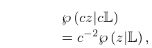
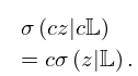
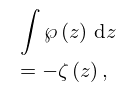
the functions are related by … ►When it is important to display the lattice with the functions they are denoted by

\wp\left(z|\mathbb{L}\right)

,

\zeta\left(z|\mathbb{L}\right)

, and

\sigma\left(z|\mathbb{L}\right)

, respectively. … ►If

2\omega_{1}

,

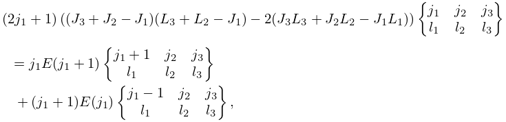
2\omega_{3}

is any pair of generators of

\mathbb{L}

, and

\omega_{2}

is defined by (23.2.1), then …

L’Hôpital rule

1—10 of 134 matching pages

1: 25.15 Dirichlet $L$ -functions

§25.15 Dirichlet $L$ -functions

§25.15(i) Definitions and Basic Properties

§25.15(ii) Zeros

2: 3.5 Quadrature

§3.5(i) Trapezoidal Rules

§3.5(ii) Simpson’s Rule

§3.5(iv) Interpolatory Quadrature Rules

3: 1.4 Calculus of One Variable

Chain Rule

L’Hôpital’s Rule

4: 3.2 Linear Algebra

5: 34.5 Basic Properties: $\mathit{6j}$ Symbol

6: 18.4 Graphics

7: 23.10 Addition Theorems and Other Identities

8: 18.36 Miscellaneous Polynomials

§18.36(v) Non-Classical Laguerre Polynomials $L^{(-k)}_{n}\left(x\right)$ , $k=1,2\dots$

9: 23.14 Integrals

10: 23.2 Definitions and Periodic Properties

L’Hôpital rule

1—10 of 134 matching pages

1: 25.15 Dirichlet L -functions

§25.15 Dirichlet L -functions

§25.15(i) Definitions and Basic Properties

§25.15(ii) Zeros

2: 3.5 Quadrature

§3.5(i) Trapezoidal Rules

§3.5(ii) Simpson’s Rule

§3.5(iv) Interpolatory Quadrature Rules

3: 1.4 Calculus of One Variable

Chain Rule

L’Hôpital’s Rule

4: 3.2 Linear Algebra

5: 34.5 Basic Properties: 6 ⁢ j Symbol

6: 18.4 Graphics

7: 23.10 Addition Theorems and Other Identities

8: 18.36 Miscellaneous Polynomials

§18.36(v) Non-Classical Laguerre Polynomials L n ( − k ) ⁡ ( x ) , k = 1 , 2 ⁢ …

9: 23.14 Integrals

10: 23.2 Definitions and Periodic Properties

1: 25.15 Dirichlet $L$ -functions

§25.15 Dirichlet $L$ -functions

5: 34.5 Basic Properties: $\mathit{6j}$ Symbol

§18.36(v) Non-Classical Laguerre Polynomials $L^{(-k)}_{n}\left(x\right)$ , $k=1,2\dots$