L%20orthornormal%20basis

SearchAdvancedHelp

The term"orthornorm" was not found.Possible alternative term: "orthonorm".

(0.003 seconds)

1—10 of 199 matching pages

1: 23.14 Integrals

… ►

23.14.1 $$\int \mathrm{\wp }\left(z\right)dz=-\zeta \left(z\right),$$

ⓘ

Symbols:

$\mathrm{\wp }\left(z\right)$ (= $\mathrm{\wp }\left(z|𝕃\right)$ = $\mathrm{\wp }(z;g_2,g_3)$): Weierstrass $\mathrm{\wp }$-function, $\zeta \left(z\right)$ (= $\zeta \left(z|𝕃\right)$ = $\zeta (z;g_2,g_3)$): Weierstrass zeta function, $dx$: differential of $x$ , $\int$: integral, $𝕃$: lattice and $z$: complex

A&S Ref:

18.6.1

Permalink:

http://dlmf.nist.gov/23.14.E1

Encodings:

pMML, png, TeX

See also:

Annotations for §23.14 and Ch.23

►

23.14.2 $$\int {\mathrm{\wp }}^2\left(z\right)dz=\frac{1}{6}{\mathrm{\wp }}^{\prime }\left(z\right)+\frac{1}{12}{g}_{2}z,$$

ⓘ

Symbols:

$\mathrm{\wp }\left(z\right)$ (= $\mathrm{\wp }\left(z|𝕃\right)$ = $\mathrm{\wp }(z;g_2,g_3)$): Weierstrass $\mathrm{\wp }$-function, $g_j$: Weierstrass lattice invariants $g_2$, $g_3$ , $dx$: differential of $x$ , $\int$: integral, $𝕃$: lattice and $z$: complex

A&S Ref:

18.7.1

Permalink:

http://dlmf.nist.gov/23.14.E2

Encodings:

pMML, png, TeX

See also:

Annotations for §23.14 and Ch.23

►

23.14.3 $$\int {\mathrm{\wp }}^3\left(z\right)dz=\frac{1}{120}{\mathrm{\wp }}^{\prime \prime \prime }\left(z\right)-\frac{3}{20}{g}_2\zeta \left(z\right)+\frac{1}{10}{g}_{3}z.$$

ⓘ

Symbols:

$\mathrm{\wp }\left(z\right)$ (= $\mathrm{\wp }\left(z|𝕃\right)$ = $\mathrm{\wp }(z;g_2,g_3)$): Weierstrass $\mathrm{\wp }$-function, $g_j$: Weierstrass lattice invariants $g_2$, $g_3$ , $\zeta \left(z\right)$ (= $\zeta \left(z|𝕃\right)$ = $\zeta (z;g_2,g_3)$): Weierstrass zeta function, $dx$: differential of $x$ , $\int$: integral, $𝕃$: lattice and $z$: complex

A&S Ref:

18.7.2

Permalink:

http://dlmf.nist.gov/23.14.E3

Encodings:

pMML, png, TeX

See also:

Annotations for §23.14 and Ch.23

…

2: 23.9 Laurent and Other Power Series

… ►

23.9.1 $$c_n=(2n-1)\sum _{w\in 𝕃\setminus \{0\}}{w}^{-2n},$$ $n=2,3,4,\mathrm{\dots }$.

ⓘ

Symbols:

$\in$: element of, $\setminus$: set subtraction, $𝕃$: lattice, $n$: integer and $c_n$

Referenced by:

§20.6

Permalink:

http://dlmf.nist.gov/23.9.E1

Encodings:

pMML, png, TeX

See also:

Annotations for §23.9 and Ch.23

… ►

23.9.2 $$\mathrm{\wp }\left(z\right)=\frac{1}{z^2}+\sum _{n=2}^{\mathrm{\infty }}{c}_n{z}^{2n-2},$$ ,

ⓘ

Symbols:

$\mathrm{\wp }\left(z\right)$ (= $\mathrm{\wp }\left(z|𝕃\right)$ = $\mathrm{\wp }(z;g_2,g_3)$): Weierstrass $\mathrm{\wp }$-function, $𝕃$: lattice, $n$: integer, $z$: complex and $c_n$

A&S Ref:

18.5.1

Referenced by:

§23.9, §23.9

Permalink:

http://dlmf.nist.gov/23.9.E2

Encodings:

pMML, png, TeX

See also:

Annotations for §23.9 and Ch.23

►

23.9.3 $$\zeta \left(z\right)=\frac{1}{z}-\sum _{n=2}^{\mathrm{\infty }}\frac{c_n}{2n-1}{z}^{2n-1},$$ .

ⓘ

Symbols:

$\zeta \left(z\right)$ (= $\zeta \left(z|𝕃\right)$ = $\zeta (z;g_2,g_3)$): Weierstrass zeta function, $𝕃$: lattice, $n$: integer, $z$: complex and $c_n$

A&S Ref:

18.5.5

Referenced by:

§23.9

Permalink:

http://dlmf.nist.gov/23.9.E3

Encodings:

pMML, png, TeX

See also:

Annotations for §23.9 and Ch.23

… ►

$c_2={\displaystyle \frac{1}{20}}{g}_2,$

… ►

23.9.7 $$\sigma \left(z\right)=\sum _{m,n=0}^{\mathrm{\infty }}{a}_{m,n}{(10c_2)}^m{(56c_3)}^n\frac{z^{4m+6n+1}}{(4m+6n+1)!},$$

ⓘ

Symbols:

$\sigma \left(z\right)$ (= $\sigma \left(z|𝕃\right)$ = $\sigma (z;g_2,g_3)$): Weierstrass sigma function, $!$: factorial (as in $n!$), $𝕃$: lattice, $n$: integer, $m$: integer, $z$: complex, $c_n$ and $a_{m,n}$: coefficients

A&S Ref:

18.5.6

Referenced by:

§23.9

Permalink:

http://dlmf.nist.gov/23.9.E7

Encodings:

pMML, png, TeX

See also:

Annotations for §23.9 and Ch.23

…

3: 11.14 Tables

… ►

Abramowitz and Stegun (1964, Chapter 12) tabulates ${𝐇}_n\left(x\right)$, ${𝐇}_n\left(x\right)-Y_n\left(x\right)$, and $I_n\left(x\right)-{𝐋}_n\left(x\right)$ for $n=0,1$ and $x=0(.1)5$, $x^{-1}=0(.01)0.2$ to 6D or 7D.

►

Agrest et al. (1982) tabulates ${𝐇}_n\left(x\right)$ and ${\mathrm{e}}^{-x}{𝐋}_n\left(x\right)$ for $n=0,1$ and $x=0(.001)5(.005)15(.01)100$ to 11D.

►

Barrett (1964) tabulates ${𝐋}_n\left(x\right)$ for $n=0,1$ and $x=0.2(.005)4(.05)10(.1)19.2$ to 5 or 6S, $x=6(.25)59.5(.5)100$ to 2S.

… ►

Zhang and Jin (1996) tabulates ${𝐇}_n\left(x\right)$ and ${𝐋}_n\left(x\right)$ for $n=-4(1)3$ and $x=0(1)20$ to 8D or 7S.

… ►

Agrest et al. (1982) tabulates ${\int }_0^x{𝐇}_0\left(t\right)dt$ and ${\mathrm{e}}^{-x}{\int }_0^x{𝐋}_0\left(t\right)dt$ for $x=0(.001)5(.005)15(.01)100$ to 11D.

…

4: 20 Theta Functions

Chapter 20 Theta Functions

…

5: 18.39 Applications in the Physical Sciences

… ►where ${\mathrm{L}}^2$ is the (squared) angular momentum operator (14.30.12). … ►with an infinite set of orthonormal $L^2$ eigenfunctions … ►is tridiagonalized in the complete $L^2$ non-orthogonal (with measure $dr$, $r\in [0,\mathrm{\infty })$) basis of Laguerre functions: … ►For either sign of $Z$, and $s$ chosen such that $n+l+1+(2Z/s)>0$, $n=0,1,2,\mathrm{\dots }$, truncation of the basis to $N$ terms, with $x_i^N\in [-1,1]$, the discrete eigenvectors are the orthonormal $L^2$ functions …This equivalent quadrature relationship, see Heller et al. (1973), Yamani and Reinhardt (1975), allows extraction of scattering information from the finite dimensional $L^2$ functions of (18.39.53), provided that such information involves potentials, or projections onto $L^2$ functions, exactly expressed, or well approximated, in the finite basis of (18.39.44). …

6: 18.5 Explicit Representations

… ►Similarly in the cases of the ultraspherical polynomials $C_n^{(\lambda )}\left(x\right)$ and the Laguerre polynomials $L_n^{(\alpha )}\left(x\right)$ we assume that $\lambda >-\frac{1}{2},\lambda \ne 0$, and $\alpha >-1$, unless stated otherwise. … ►

$L_0\left(x\right)=1,$

… ►

$L_6\left(x\right)=\frac{1}{720}{x}^6-\frac{1}{20}{x}^5+\frac{5}{8}{x}^4-\frac{10}{3}{x}^3+\frac{15}{2}{x}^2-6x+1.$

►

$L_0^{(\alpha )}\left(x\right)=1,$

►

$L_1^{(\alpha )}\left(x\right)=-x+\alpha +1,$

…

7: 25.15 Dirichlet $L$-functions

§25.15 Dirichlet $L$-functions

►

§25.15(i) Definitions and Basic Properties

►The notation $L(s,\chi )$ was introduced by Dirichlet (1837) for the meromorphic continuation of the function defined by the series … … ►

§25.15(ii) Zeros

…

8: 25.12 Polylogarithms

… ►Other notations and names for ${\mathrm{Li}}_2\left(z\right)$ include $S_2(z)$ (Kölbig et al. (1970)), Spence function $\mathrm{Sp}(z)$ (’t Hooft and Veltman (1979)), and ${\mathrm{L}}_2(z)$ (Maximon (2003)). … ►

►►

Figure 25.12.1: Dilogarithm function ${\mathrm{Li}}_2\left(x\right)$, Magnify

►

►

►

Figure 25.12.2: Absolute value of the dilogarithm function $\left|{\mathrm{Li}}_2\left(x+\mathrm{i}y\right)\right|$, $-20\le x\le 20$, $-20\le y\le 20$. … Magnify 3D Help

…

9: 23.21 Physical Applications

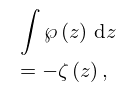
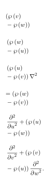
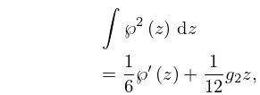
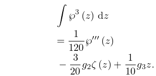
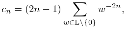
… ►In §22.19(ii) it is noted that Jacobian elliptic functions provide a natural basis of solutions for problems in Newtonian classical dynamics with quartic potentials in canonical form $(1-x^2)(1-k^2{x}^2)$. … ►

23.21.1 $$\frac{x^2}{\rho -e_1}+\frac{y^2}{\rho -e_2}+\frac{z^2}{\rho -e_3}=1,$$

ⓘ

Symbols:

$e_j$: Weierstrass lattice roots, $𝕃$: lattice, $x$: real part of $z$ , $y$: imaginary part of $z$ , $z$: complex and $\rho$: roots

Permalink:

http://dlmf.nist.gov/23.21.E1

Encodings:

pMML, png, TeX

See also:

Annotations for §23.21(iii), §23.21 and Ch.23

… ►

23.21.3 $$f(\rho )=2{\left((\rho -e_1)(\rho -e_2)(\rho -e_3)\right)}^{1/2}.$$

ⓘ

Symbols:

$e_j$: Weierstrass lattice roots, $𝕃$: lattice, $\rho$: roots and $f(\rho )$: function

Permalink:

http://dlmf.nist.gov/23.21.E3

Encodings:

pMML, png, TeX

See also:

Annotations for §23.21(iii), §23.21 and Ch.23

… ►

23.21.5 $$\left(\mathrm{\wp }\left(v\right)-\mathrm{\wp }\left(w\right)\right)\left(\mathrm{\wp }\left(w\right)-\mathrm{\wp }\left(u\right)\right)\left(\mathrm{\wp }\left(u\right)-\mathrm{\wp }\left(v\right)\right){\nabla }^2=\left(\mathrm{\wp }\left(w\right)-\mathrm{\wp }\left(v\right)\right)\frac{{\partial }^2}{{\partial u}^2}+\left(\mathrm{\wp }\left(u\right)-\mathrm{\wp }\left(w\right)\right)\frac{{\partial }^2}{{\partial v}^2}+\left(\mathrm{\wp }\left(v\right)-\mathrm{\wp }\left(u\right)\right)\frac{{\partial }^2}{{\partial w}^2}.$$

ⓘ

Symbols:

$\mathrm{\wp }\left(z\right)$ (= $\mathrm{\wp }\left(z|𝕃\right)$ = $\mathrm{\wp }(z;g_2,g_3)$): Weierstrass $\mathrm{\wp }$-function, $\frac{\partial f}{\partial x}$: partial derivative of $f$ with respect to $x$ , $\partial x$: partial differential of $x$ , $𝕃$: lattice, $u$: change of variable, $v$: change of variable and $w$: change of variable

Permalink:

http://dlmf.nist.gov/23.21.E5

Encodings:

pMML, png, TeX

See also:

Annotations for §23.21(iii), §23.21 and Ch.23

…

10: 18.4 Graphics

… ►

►►

Figure 18.4.5: Laguerre polynomials $L_n\left(x\right)$, $n=1,2,3,4,5$. Magnify

►

►►

Figure 18.4.6: Laguerre polynomials $L_3^{(\alpha )}\left(x\right)$, $\alpha =0,1,2,3,4$. Magnify

… ►

►

►

Figure 18.4.8: Laguerre polynomials $L_3^{(\alpha )}\left(x\right)$, $0\le \alpha \le 3$, $0\le x\le 10$. Magnify 3D Help

►

►

►

Figure 18.4.9: Laguerre polynomials $L_4^{(\alpha )}\left(x\right)$, $0\le \alpha \le 3$, $0\le x\le 10$. Magnify 3D Help