Jacobi function

SearchAdvancedHelp

(0.009 seconds)

21—30 of 121 matching pages

21: 20.2 Definitions and Periodic Properties

… ►

§20.2(i) Fourier Series

►

20.2.1 $${\theta }_1\left(z\right|\tau )={\theta }_1(z,q)=2\sum _{n=0}^{\mathrm{\infty }}{(-1)}^n{q}^{{(n+\frac{1}{2})}^2}\sin \left((2n+1)z\right),$$

ⓘ

Symbols:

${\theta }_j(z,q)$: theta function, ${\theta }_j\left(z\right|\tau )$: theta function, $\sin z$: sine function, $n$: integer, $z$: complex, $\tau$: lattice parameter and $q$: nome

A&S Ref:

16.27.1

Referenced by:

§20.14, §20.2(i)

Permalink:

http://dlmf.nist.gov/20.2.E1

Encodings:

pMML, png, TeX

See also:

Annotations for §20.2(i), §20.2 and Ch.20

►

20.2.2 $${\theta }_2\left(z\right|\tau )={\theta }_2(z,q)=2\sum _{n=0}^{\mathrm{\infty }}{q}^{{(n+\frac{1}{2})}^2}\cos \left((2n+1)z\right),$$

ⓘ

Symbols:

${\theta }_j(z,q)$: theta function, ${\theta }_j\left(z\right|\tau )$: theta function, $\cos z$: cosine function, $n$: integer, $z$: complex, $\tau$: lattice parameter and $q$: nome

A&S Ref:

16.27.2

Permalink:

http://dlmf.nist.gov/20.2.E2

Encodings:

pMML, png, TeX

See also:

Annotations for §20.2(i), §20.2 and Ch.20

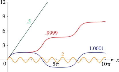
… ►For fixed $\tau$, each ${\theta }_j\left(z\right|\tau )$ is an entire function of $z$ with period $2\pi$; ${\theta }_1\left(z\right|\tau )$ is odd in $z$ and the others are even. For fixed $z$, each of ${\theta }_1\left(z\right|\tau )/\sin z$, ${\theta }_2\left(z\right|\tau )/\cos z$, ${\theta }_3\left(z\right|\tau )$, and ${\theta }_4\left(z\right|\tau )$ is an analytic function of $\tau$ for $\mathrm{\Im }\tau >0$, with a natural boundary $\mathrm{\Im }\tau =0$, and correspondingly, an analytic function of $q$ for with a natural boundary $\left|q\right|=1$. …

22: 15.9 Relations to Other Functions

… ►

Jacobi

… ►

§15.9(ii) Jacobi Function

… ►

15.9.11 $${\varphi }_{\lambda }^{(\alpha ,\beta )}\left(t\right)=F(\genfrac{}{}{0pt}{}{\frac{1}{2}(\alpha +\beta +1-\mathrm{i}\lambda ),\frac{1}{2}(\alpha +\beta +1+\mathrm{i}\lambda )}{\alpha +1};-{\sinh }^{2}t).$$

ⓘ

Defines:

${\varphi }_{\lambda }^{(\alpha ,\beta )}\left(t\right)$: Jacobi function

Symbols:

$F(a,b;c;z)$ or $F(\genfrac{}{}{0pt}{}{a,b}{c};z)$: $={}_2{}^{}F_1^{}(a,b;c;z)$ Gauss’ hypergeometric function, $\sinh z$: hyperbolic sine function and $\mathrm{i}$: imaginary unit

Permalink:

http://dlmf.nist.gov/15.9.E11

Encodings:

pMML, png, TeX

See also:

Annotations for §15.9(ii), §15.9 and Ch.15

… ►

15.9.12 $$\tilde{f}(\lambda )={\int }_0^{\mathrm{\infty }}f(t){\varphi }_{\lambda }^{(\alpha ,\beta )}\left(t\right){(2\sinh t)}^{2\alpha +1}{(2\cosh t)}^{2\beta +1}dt,$$

ⓘ

Symbols:

${\varphi }_{\lambda }^{(\alpha ,\beta )}\left(t\right)$: Jacobi function, $dx$: differential of $x$ , $\cosh z$: hyperbolic cosine function, $\sinh z$: hyperbolic sine function, $\int$: integral and $f(t)$: function

Permalink:

http://dlmf.nist.gov/15.9.E12

Encodings:

pMML, png, TeX

See also:

Annotations for §15.9(ii), §15.9 and Ch.15

►with inverse …

23: 22.20 Methods of Computation

… ►

§22.20(vi) Related Functions

… ►Jacobi’s epsilon function can be computed from its representation (22.16.30) in terms of theta functions and complete elliptic integrals; compare §20.14. Jacobi’s zeta function can then be found by use of (22.16.32). … ►For additional information on methods of computation for the Jacobi and related functions, see the introductory sections in the following books: Lawden (1989), Curtis (1964b), Milne-Thomson (1950), and Spenceley and Spenceley (1947). …

24: 10.35 Generating Function and Associated Series

… ►Jacobi–Anger expansions: for $z,\theta \in ℂ$, …

25: 29.18 Mathematical Applications

… ►

29.18.6 $$\frac{d^2{u}_2}{{d\beta }^2}+(h-\nu (\nu +1)k^2{\mathrm{sn}}^2(\beta ,k))u_2=0,$$

ⓘ

Symbols:

$\mathrm{sn}(z,k)$: Jacobian elliptic function, $\frac{df}{dx}$: derivative of $f$ with respect to $x$ , $h$: real parameter, $k$: real parameter, $\nu$: real parameter, $\beta$: sphero-conal coordinate and $u_j$: solutions

Referenced by:

§29.18(i)

Permalink:

http://dlmf.nist.gov/29.18.E6

Encodings:

pMML, png, TeX

See also:

Annotations for §29.18(i), §29.18 and Ch.29

►

29.18.7 $$\frac{d^2{u}_3}{{d\gamma }^2}+(h-\nu (\nu +1)k^2{\mathrm{sn}}^2(\gamma ,k))u_3=0,$$

ⓘ

Symbols:

$\mathrm{sn}(z,k)$: Jacobian elliptic function, $\frac{df}{dx}$: derivative of $f$ with respect to $x$ , $h$: real parameter, $k$: real parameter, $\nu$: real parameter, $\gamma$: sphero-conal coordinate and $u_j$: solutions

Referenced by:

§29.18(i)

Permalink:

http://dlmf.nist.gov/29.18.E7

Encodings:

pMML, png, TeX

See also:

Annotations for §29.18(i), §29.18 and Ch.29

…

26: 20.1 Special Notation

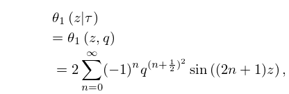
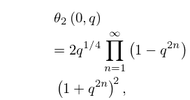
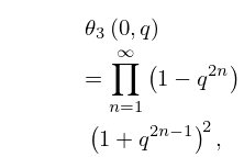
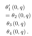
… ►The main functions treated in this chapter are the theta functions ${\theta }_j\left(z\right|\tau )={\theta }_j(z,q)$ where $j=1,2,3,4$ and $q={\mathrm{e}}^{\mathrm{i}\pi \tau }$. … ►Primes on the $\theta$ symbols indicate derivatives with respect to the argument of the $\theta$ function. … ►Jacobi’s original notation: $\mathrm{\Theta }(z|\tau )$, ${\mathrm{\Theta }}_1(z|\tau )$, $\mathrm{H}(z|\tau )$, ${\mathrm{H}}_1(z|\tau )$, respectively, for ${\theta }_4\left(u\right|\tau )$, ${\theta }_3\left(u\right|\tau )$, ${\theta }_1\left(u\right|\tau )$, ${\theta }_2\left(u\right|\tau )$, where $u=z/{\theta }_3^2\left(0\right|\tau )$. … ►Neville’s notation: ${\theta }_s(z|\tau )$, ${\theta }_c(z|\tau )$, ${\theta }_d(z|\tau )$, ${\theta }_n(z|\tau )$, respectively, for ${\theta }_3^2\left(0\right|\tau ){\theta }_1\left(u\right|\tau )/{\theta }_1^{\prime }\left(0\right|\tau )$, ${\theta }_2\left(u\right|\tau )/{\theta }_2\left(0\right|\tau )$, ${\theta }_3\left(u\right|\tau )/{\theta }_3\left(0\right|\tau )$, ${\theta }_4\left(u\right|\tau )/{\theta }_4\left(0\right|\tau )$, where again $u=z/{\theta }_3^2\left(0\right|\tau )$. … ►McKean and Moll’s notation: ${\vartheta }_j(z|\tau )={\theta }_j\left(\pi z\right|\tau )$, $j=1,2,3,4$. …

27: 22.19 Physical Applications

… ►

§22.19(i) Classical Dynamics: The Pendulum

… ►

22.19.2 $$\sin \left(\frac{1}{2}\theta (t)\right)=\sin \left(\frac{1}{2}\alpha \right)\mathrm{sn}(t+K,\sin \left(\frac{1}{2}\alpha \right)),$$

ⓘ

Symbols:

$\mathrm{sn}(z,k)$: Jacobian elliptic function, $K\left(k\right)$: Legendre’s complete elliptic integral of the first kind, $\sin z$: sine function, $\theta (t)$: angular displacement and $\alpha$: initial displacement

Referenced by:

§22.19(i), §22.19(i), Erratum (V1.0.8) for Equation (22.19.2)

Permalink:

http://dlmf.nist.gov/22.19.E2

Encodings:

pMML, png, TeX

Errata (effective with 1.0.8):

Originally the first argument to the function $\mathrm{sn}$ was given incorrectly as $t$. The correct argument is $t+K$.

Reported 2014-03-05 by Svante Janson

See also:

Annotations for §22.19(i), §22.19 and Ch.22

… ►

22.19.3 $$\theta (t)=2\mathrm{am}(t\sqrt{E/2},\sqrt{2/E}),$$

ⓘ

Symbols:

$\mathrm{am}(x,k)$: Jacobi’s amplitude function, $\theta (t)$: angular displacement and $E$: energy

Referenced by:

§22.19(i), §22.19(i), Erratum (V1.0.8) for Equation (22.19.3)

Permalink:

http://dlmf.nist.gov/22.19.E3

Encodings:

pMML, png, TeX

Errata (effective with 1.0.8):

Originally the first argument to the function $\mathrm{am}$ was given incorrectly as $t$. The correct argument is $t\sqrt{E/2}$.

Reported 2014-03-05 by Svante Janson

See also:

Annotations for §22.19(i), §22.19 and Ch.22

… ►

►►

Figure 22.19.1: Jacobi’s amplitude function $\mathrm{am}(x,k)$ for $0\le x\le 10\pi$ and $k=0.5,0.9999,1.0001,2$. … Magnify

… ►

22.19.8 $$x(t)=a\mathrm{dn}(t\sqrt{\eta },k).$$

ⓘ

Symbols:

$\mathrm{dn}(z,k)$: Jacobian elliptic function, $k$: modulus, $x(t)$: coordinate, $t$: time, $a$: displacement and $\eta$: parameter

Referenced by:

Erratum (V1.0.9) for Equations (22.19.6), (22.19.7), (22.19.8), (22.19.9)

Permalink:

http://dlmf.nist.gov/22.19.E8

Encodings:

pMML, png, TeX

See also:

Annotations for §22.19(ii), §22.19(ii), §22.19 and Ch.22

…

28: 20.4 Values at $z$ = 0

… ►

20.4.3 $${\theta }_2(0,q)=2q^{1/4}\prod _{n=1}^{\mathrm{\infty }}\left(1-q^{2n}\right){\left(1+q^{2n}\right)}^2,$$

ⓘ

Symbols:

${\theta }_j(z,q)$: theta function, $n$: integer and $q$: nome

Referenced by:

(20.10.3)

Permalink:

http://dlmf.nist.gov/20.4.E3

Encodings:

pMML, png, TeX

See also:

Annotations for §20.4(i), §20.4 and Ch.20

►

20.4.4 $${\theta }_3(0,q)=\prod _{n=1}^{\mathrm{\infty }}\left(1-q^{2n}\right){\left(1+q^{2n-1}\right)}^2,$$

ⓘ

Symbols:

${\theta }_j(z,q)$: theta function, $n$: integer and $q$: nome

Referenced by:

(20.10.2)

Permalink:

http://dlmf.nist.gov/20.4.E4

Encodings:

pMML, png, TeX

See also:

Annotations for §20.4(i), §20.4 and Ch.20

►

20.4.5 $${\theta }_4(0,q)=\prod _{n=1}^{\mathrm{\infty }}\left(1-q^{2n}\right){\left(1-q^{2n-1}\right)}^2.$$

ⓘ

Symbols:

${\theta }_j(z,q)$: theta function, $n$: integer and $q$: nome

Referenced by:

(20.10.1)

Permalink:

http://dlmf.nist.gov/20.4.E5

Encodings:

pMML, png, TeX

See also:

Annotations for §20.4(i), §20.4 and Ch.20

►

Jacobi’s Identity

►

20.4.6 $${\theta }_1^{\prime }(0,q)={\theta }_2(0,q){\theta }_3(0,q){\theta }_4(0,q).$$

ⓘ

Symbols:

${\theta }_j(z,q)$: theta function and $q$: nome

A&S Ref:

16.28.6

Referenced by:

§20.9(i)

Permalink:

http://dlmf.nist.gov/20.4.E6

Encodings:

pMML, png, TeX

See also:

Annotations for §20.4(i), §20.4(i), §20.4 and Ch.20

…

29: 23.15 Definitions

… ►

23.15.6 $$\lambda \left(\tau \right)=\frac{{\theta }_2^4(0,q)}{{\theta }_3^4(0,q)};$$

ⓘ

Defines:

$\lambda \left(\tau \right)$: elliptic modular function

Symbols:

${\theta }_j(z,q)$: theta function, $q$: nome and $\tau$: complex variable

Referenced by:

§20.9(ii), §23.17(iii)

Permalink:

http://dlmf.nist.gov/23.15.E6

Encodings:

pMML, png, TeX

See also:

Annotations for §23.15(ii), §23.15(ii), §23.15 and Ch.23

… ►

23.15.7 $$J\left(\tau \right)=\frac{{\left({\theta }_2^8(0,q)+{\theta }_3^8(0,q)+{\theta }_4^8(0,q)\right)}^3}{54{\left({\theta }_1^{\prime }(0,q)\right)}^8},$$

ⓘ

Defines:

$J\left(\tau \right)$: Klein’s complete invariant

Symbols:

${\theta }_j(z,q)$: theta function, $q$: nome and $\tau$: complex variable

Permalink:

http://dlmf.nist.gov/23.15.E7

Encodings:

pMML, png, TeX

See also:

Annotations for §23.15(ii), §23.15(ii), §23.15 and Ch.23

… ►

23.15.8 $${\theta }_1^{\prime }(0,q)={\partial {\theta }_1(z,q)/\partial z|}_{z=0}.$$

ⓘ

Symbols:

${\theta }_j(z,q)$: theta function, $\frac{\partial f}{\partial x}$: partial derivative of $f$ with respect to $x$ , $\partial x$: partial differential of $x$ , $q$: nome and $z$: complex

Permalink:

http://dlmf.nist.gov/23.15.E8

Encodings:

pMML, png, TeX

See also:

Annotations for §23.15(ii), §23.15(ii), §23.15 and Ch.23

… ►

23.15.9 $$\eta \left(\tau \right)={\left(\frac{1}{2}{\theta }_1^{\prime }(0,q)\right)}^{1/3}={\mathrm{e}}^{\mathrm{i}\pi \tau /12}{\theta }_3\left(\frac{1}{2}\pi (1+\tau )\right|3\tau ).$$

ⓘ

Symbols:

$\eta \left(\tau \right)$: Dedekind’s eta function (or Dedekind modular function), ${\theta }_j(z,q)$: theta function, ${\theta }_j\left(z\right|\tau )$: theta function, $\pi$: the ratio of the circumference of a circle to its diameter, $\mathrm{e}$: base of natural logarithm, $\mathrm{i}$: imaginary unit, $q$: nome and $\tau$: complex variable

Referenced by:

§23.15(ii), §23.15(ii), §23.17(iii)

Permalink:

http://dlmf.nist.gov/23.15.E9

Encodings:

pMML, png, TeX

See also:

Annotations for §23.15(ii), §23.15(ii), §23.15 and Ch.23

…

30: 14.3 Definitions and Hypergeometric Representations

… ►

§14.3(iv) Relations to Other Functions

►In terms of the Gegenbauer function $C_{\alpha }^{(\beta )}\left(x\right)$ and the Jacobi function ${\varphi }_{\lambda }^{(\alpha ,\beta )}\left(t\right)$ (§§15.9(iii), 15.9(ii)): … ►

14.3.23

ⓘ

Symbols:

$\mathrm{\Gamma }\left(z\right)$: gamma function, ${\varphi }_{\lambda }^{(\alpha ,\beta )}\left(t\right)$: Jacobi function, $P_{\nu }^{\mu }\left(z\right)$: associated Legendre function of the first kind, $\mathrm{arcsinh}z$: inverse hyperbolic sine function, $\mathrm{i}$: imaginary unit, $\mu$: general order, $\nu$: general degree and : real variable

Referenced by:

§14.3(iv)

Permalink:

http://dlmf.nist.gov/14.3.E23

Encodings:

pMML, png, TeX

See also:

Annotations for §14.3(iv), §14.3 and Ch.14

…