Jacobi elliptic
(0.007 seconds)
21—30 of 61 matching pages
21: 22.20 Methods of Computation
…
►To compute , , to 10D when , .
…
►Then from (22.20.5), , , .
…
►Then by using (22.7.4) we have .
►If needed, the corresponding values of and can be found subsequently by applying (22.10.4) and (22.7.2), followed by (22.10.5) and (22.7.3).
…
►
§22.20(vi) Related Functions
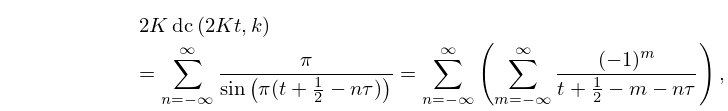
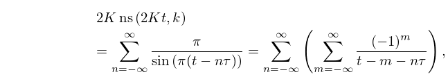
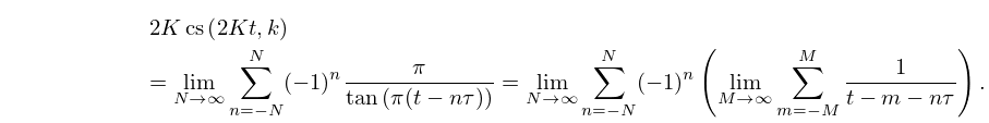
…22: 22.12 Expansions in Other Trigonometric Series and Doubly-Infinite Partial Fractions: Eisenstein Series
23: 29.17 Other Solutions
…
►They are algebraic functions of , , and , and have primitive period .
…
►Lamé–Wangerin functions are solutions of (29.2.1) with the property that is bounded on the line segment from to .
…
24: 29.12 Definitions
…
►These functions are polynomials in , , and .
…
►In the fourth column the variable and modulus of the Jacobian elliptic functions have been suppressed, and denotes a polynomial of degree in (different for each type).
…
►
Table 29.12.1: Lamé polynomials.
►
►
►
…
►With the substitution every Lamé polynomial in Table 29.12.1 can be written in the form
…
|
|
|
|
|
|
|
|
|
|
|||||||||||||||||
|---|---|---|---|---|---|---|---|---|---|---|---|---|---|---|---|---|---|---|---|---|---|---|---|---|---|
| … | |||||||||||||||||||||||||
| odd | odd | even | |||||||||||||||||||||||
| … | |||||||||||||||||||||||||
| odd | odd | odd | |||||||||||||||||||||||
25: 29.15 Fourier Series and Chebyshev Series
…
►Since (29.2.5) implies that , (29.15.1) can be rewritten in the form
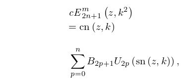
…This determines the polynomial of degree for which ; compare Table 29.12.1.
…
►
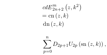
29.15.45
…
►
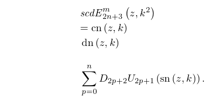
29.15.49
►
29.15.50
…
26: 22.19 Physical Applications
…
►
§22.19(i) Classical Dynamics: The Pendulum
… ►
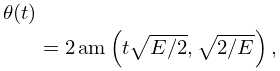
22.19.3
…
►Figure 22.19.1 shows the nature of the solutions of (22.19.3) by graphing for both , as in Figure 22.16.1, and , where it is periodic.
…
►
22.19.8
…
►Both the and solutions approach as from the appropriate directions.
…
27: 31.2 Differential Equations
28: 22.9 Cyclic Identities
29: 19.25 Relations to Other Functions
…
►
19.25.28
…
►If , then
►
19.25.30
►
19.25.31
…
►where we assume if , , or ; if , , or ; real if or ; if ; if ; if ; if .
…
30: 29.10 Lamé Functions with Imaginary Periods
…
►
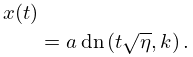
29.10.3
…
