Jacobi

SearchAdvancedHelp

(0.000 seconds)

31—40 of 126 matching pages

31: 22.3 Graphics

… ►Line graphs of the functions $\mathrm{sn}(x,k)$, $\mathrm{cn}(x,k)$, $\mathrm{dn}(x,k)$, $\mathrm{cd}(x,k)$, $\mathrm{sd}(x,k)$, $\mathrm{nd}(x,k)$, $\mathrm{dc}(x,k)$, $\mathrm{nc}(x,k)$, $\mathrm{sc}(x,k)$, $\mathrm{ns}(x,k)$, $\mathrm{ds}(x,k)$, and $\mathrm{cs}(x,k)$ for representative values of real $x$ and real $k$ illustrating the near trigonometric ($k=0$), and near hyperbolic ($k=1$) limits. 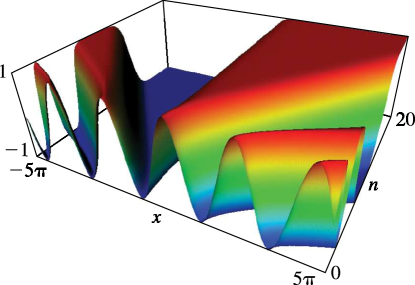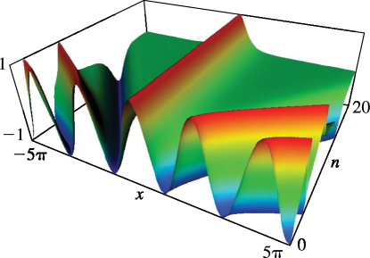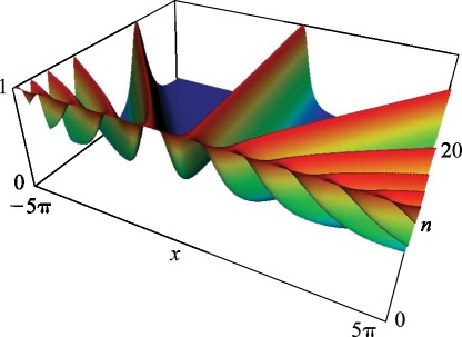… ► $\mathrm{sn}(x,k)$, $\mathrm{cn}(x,k)$, and $\mathrm{dn}(x,k)$ as functions of real arguments $x$ and $k$. … ►

►

►

Figure 22.3.13: $\mathrm{sn}(x,k)$ for $k=1-{\mathrm{e}}^{-n}$, $n=0$ to 20, $-5\pi \le x\le 5\pi$. Magnify 3D Help

►

►

►

Figure 22.3.14: $\mathrm{cn}(x,k)$ for $k=1-{\mathrm{e}}^{-n}$, $n=0$ to 20, $-5\pi \le x\le 5\pi$. Magnify 3D Help

►

►

►

Figure 22.3.15: $\mathrm{dn}(x,k)$ for $k=1-{\mathrm{e}}^{-n}$, $n=0$ to 20, $-5\pi \le x\le 5\pi$. Magnify 3D Help

…

32: 20.5 Infinite Products and Related Results

… ►

20.5.1 $${\theta }_1(z,q)=2q^{1/4}\sin z\prod _{n=1}^{\mathrm{\infty }}\left(1-q^{2n}\right)\left(1-2q^{2n}\cos \left(2z\right)+q^{4n}\right),$$

ⓘ

Symbols:

${\theta }_j(z,q)$: theta function, $\cos z$: cosine function, $\sin z$: sine function, $n$: integer, $z$: complex and $q$: nome

Referenced by:

§20.4(i), §20.5(i), §23.17(iii)

Permalink:

http://dlmf.nist.gov/20.5.E1

Encodings:

pMML, png, TeX

See also:

Annotations for §20.5(i), §20.5 and Ch.20

►

20.5.2 $${\theta }_2(z,q)=2q^{1/4}\cos z\prod _{n=1}^{\mathrm{\infty }}\left(1-q^{2n}\right)\left(1+2q^{2n}\cos \left(2z\right)+q^{4n}\right),$$

ⓘ

Symbols:

${\theta }_j(z,q)$: theta function, $\cos z$: cosine function, $n$: integer, $z$: complex and $q$: nome

Permalink:

http://dlmf.nist.gov/20.5.E2

Encodings:

pMML, png, TeX

See also:

Annotations for §20.5(i), §20.5 and Ch.20

►

20.5.3 $${\theta }_3(z,q)=\prod _{n=1}^{\mathrm{\infty }}\left(1-q^{2n}\right)\left(1+2q^{2n-1}\cos \left(2z\right)+q^{4n-2}\right),$$

ⓘ

Symbols:

${\theta }_j(z,q)$: theta function, $\cos z$: cosine function, $n$: integer, $z$: complex and $q$: nome

Referenced by:

§23.15(ii), §23.17(iii), §23.19

Permalink:

http://dlmf.nist.gov/20.5.E3

Encodings:

pMML, png, TeX

See also:

Annotations for §20.5(i), §20.5 and Ch.20

►

20.5.4 $${\theta }_4(z,q)=\prod _{n=1}^{\mathrm{\infty }}\left(1-q^{2n}\right)\left(1-2q^{2n-1}\cos \left(2z\right)+q^{4n-2}\right).$$

ⓘ

Symbols:

${\theta }_j(z,q)$: theta function, $\cos z$: cosine function, $n$: integer, $z$: complex and $q$: nome

Referenced by:

§20.4(i), §20.5(i)

Permalink:

http://dlmf.nist.gov/20.5.E4

Encodings:

pMML, png, TeX

See also:

Annotations for §20.5(i), §20.5 and Ch.20

… ►

Jacobi’s Triple Product

…

33: 18.10 Integral Representations

… ►

18.10.1 $$\frac{P_n^{(\alpha ,\alpha )}\left(\cos \theta \right)}{P_n^{(\alpha ,\alpha )}\left(1\right)}=\frac{C_n^{(\alpha +\frac{1}{2})}\left(\cos \theta \right)}{C_n^{(\alpha +\frac{1}{2})}\left(1\right)}=\frac{2^{\alpha +\frac{1}{2}}\mathrm{\Gamma }\left(\alpha +1\right)}{{\pi }^{\frac{1}{2}}\mathrm{\Gamma }\left(\alpha +\frac{1}{2}\right)}{(\sin \theta )}^{-2\alpha }{\int }_0^{\theta }\frac{\cos \left((n+\alpha +\frac{1}{2})\varphi \right)}{{(\cos \varphi -\cos \theta )}^{-\alpha +\frac{1}{2}}}d\varphi ,$$ , $\alpha >-\frac{1}{2}$.

ⓘ

Symbols:

$\mathrm{\Gamma }\left(z\right)$: gamma function, $P_n^{(\alpha ,\beta )}\left(x\right)$: Jacobi polynomial, $\pi$: the ratio of the circumference of a circle to its diameter, $\cos z$: cosine function, $dx$: differential of $x$ , $\int$: integral, $\sin z$: sine function, $C_n^{(\lambda )}\left(x\right)$: ultraspherical (or Gegenbauer) polynomial and $n$: nonnegative integer

A&S Ref:

22.10.11

Referenced by:

§18.10(i), §18.10(i)

Permalink:

http://dlmf.nist.gov/18.10.E1

Encodings:

pMML, png, TeX

See also:

Annotations for §18.10(i), §18.10(i), §18.10 and Ch.18

… ►Generalizations of (18.10.1) for $P_n^{(\alpha ,\beta )}$ are given in Gasper (1975, (6),(8)) and Koornwinder (1975a, (5.7),(5.8)). … ►

Jacobi

… ►for the Jacobi, Laguerre, and Hermite polynomials. … ►

Table 18.10.1: Classical OP’s: contour integral representations (18.10.8).

► ►►

$p_n(x)$	$g_0(x)$	$g_1(z,x)$	$g_2(z,x)$	$c$	Conditions
…

►

…

34: 18.12 Generating Functions

… ►The $z$-radii of convergence will depend on $x$, and in first instance we will assume $x\in [-1,1]$ for Jacobi, ultraspherical, Chebyshev and Legendre, $x\in [0,\mathrm{\infty })$ for Laguerre, and $x\in ℝ$ for Hermite. … ►

Jacobi

►

18.12.1 $$\frac{2^{\alpha +\beta }}{R{(1+R-z)}^{\alpha }{(1+R+z)}^{\beta }}=\sum _{n=0}^{\mathrm{\infty }}{P}_n^{(\alpha ,\beta )}\left(x\right)z^n,$$ $R=\sqrt{1-2xz+z^2}$, ,

ⓘ

Symbols:

$P_n^{(\alpha ,\beta )}\left(x\right)$: Jacobi polynomial, $z$: complex variable, $n$: nonnegative integer and $x$: real variable

A&S Ref:

22.9.1

Referenced by:

§18.12, §18.12

Permalink:

http://dlmf.nist.gov/18.12.E1

Encodings:

pMML, png, TeX

See also:

Annotations for §18.12, §18.12 and Ch.18

… ►

18.12.3_5 $$\frac{1+z}{{(1-2xz+z^2)}^{\beta +\frac{3}{2}}}=\sum _{n=0}^{\mathrm{\infty }}\frac{{\left(2\beta +2\right)}_n}{{\left(\beta +1\right)}_n}{P}_n^{(\beta +1,\beta )}\left(x\right)z^n,$$ ,

ⓘ

Symbols:

$P_n^{(\alpha ,\beta )}\left(x\right)$: Jacobi polynomial, ${\left(a\right)}_n$: Pochhammer’s symbol (or shifted factorial), $z$: complex variable, $n$: nonnegative integer and $x$: real variable

Proof sketch:

Substitute $\alpha =\beta +1$ in (18.12.3) and use (15.4.6).

Referenced by:

§18.12, §18.12, Erratum (V1.2.0) Section 18.12

Permalink:

http://dlmf.nist.gov/18.12.E3_5

Encodings:

pMML, png, TeX

Addition (effective with 1.2.0):

This equation was added.

See also:

Annotations for §18.12, §18.12 and Ch.18

… ►

18.12.4 $${(1-2xz+z^2)}^{-\lambda }=\sum _{n=0}^{\mathrm{\infty }}{C}_n^{(\lambda )}\left(x\right)z^n=\sum _{n=0}^{\mathrm{\infty }}\frac{{\left(2\lambda \right)}_n}{{\left(\lambda +\frac{1}{2}\right)}_n}{P}_n^{(\lambda -\frac{1}{2},\lambda -\frac{1}{2})}\left(x\right)z^n,$$ .

ⓘ

Symbols:

$P_n^{(\alpha ,\beta )}\left(x\right)$: Jacobi polynomial, ${\left(a\right)}_n$: Pochhammer’s symbol (or shifted factorial), $C_n^{(\lambda )}\left(x\right)$: ultraspherical (or Gegenbauer) polynomial, $z$: complex variable, $n$: nonnegative integer and $x$: real variable

A&S Ref:

22.9.3

Referenced by:

§18.12, §18.18(viii)

Permalink:

http://dlmf.nist.gov/18.12.E4

Encodings:

pMML, png, TeX

See also:

Annotations for §18.12, §18.12 and Ch.18

…

35: 18.8 Differential Equations

… ►

Table 18.8.1: Classical OP’s: differential equations $A(x)f^{\prime \prime }(x)+B(x)f^{\prime }(x)+C(x)f(x)+{\lambda }_{n}f(x)=0$.

► ►►►►►

#	$f(x)$	$A(x)$	$B(x)$	$C(x)$	${\lambda }_n$
1	$P_n^{(\alpha ,\beta )}\left(x\right)$	$1-x^2$	$\beta -\alpha -(\alpha +\beta +2)x$	0	$n(n+\alpha +\beta +1)$
2	$\begin{array}{c}{\left(\sin \frac{1}{2}x\right)}^{\alpha +\frac{1}{2}}{\left(\cos \frac{1}{2}x\right)}^{\beta +\frac{1}{2}}\\ \times P_n^{(\alpha ,\beta )}\left(\cos x\right)\end{array}$	$1$	$0$	${\displaystyle \frac{\frac{1}{4}-{\alpha }^2}{4{\sin }^2\frac{1}{2}x}}+{\displaystyle \frac{\frac{1}{4}-{\beta }^2}{4{\cos }^2\frac{1}{2}x}}$	${\left(n+\frac{1}{2}(\alpha +\beta +1)\right)}^2$
3	${(\sin x)}^{\alpha +\frac{1}{2}}{P}_n^{(\alpha ,\alpha )}\left(\cos x\right)$	$1$	$0$	$(\frac{1}{4}-{\alpha }^2)/{\sin }^{2}x$	${(n+\alpha +\frac{1}{2})}^2$
…

►

…

36: 22.10 Maclaurin Series

… ►

22.10.1 $$\mathrm{sn}(z,k)=z-\left(1+k^2\right)\frac{z^3}{3!}+\left(1+14k^2+k^4\right)\frac{z^5}{5!}-\left(1+135k^2+135k^4+k^6\right)\frac{z^7}{7!}+O\left(z^9\right),$$

ⓘ

Symbols:

$O\left(x\right)$: order not exceeding, $\mathrm{sn}(z,k)$: Jacobian elliptic function, $!$: factorial (as in $n!$), $z$: complex and $k$: modulus

A&S Ref:

16.22.1

Permalink:

http://dlmf.nist.gov/22.10.E1

Encodings:

pMML, png, TeX

See also:

Annotations for §22.10(i), §22.10 and Ch.22

►

22.10.2 $$\mathrm{cn}(z,k)=1-\frac{z^2}{2!}+\left(1+4k^2\right)\frac{z^4}{4!}-\left(1+44k^2+16k^4\right)\frac{z^6}{6!}+O\left(z^8\right),$$

ⓘ

Symbols:

$O\left(x\right)$: order not exceeding, $\mathrm{cn}(z,k)$: Jacobian elliptic function, $!$: factorial (as in $n!$), $z$: complex and $k$: modulus

A&S Ref:

16.22.2

Permalink:

http://dlmf.nist.gov/22.10.E2

Encodings:

pMML, png, TeX

See also:

Annotations for §22.10(i), §22.10 and Ch.22

►

22.10.3 $$\mathrm{dn}(z,k)=1-k^2\frac{z^2}{2!}+k^2\left(4+k^2\right)\frac{z^4}{4!}-k^2\left(16+44k^2+k^4\right)\frac{z^6}{6!}+O\left(z^8\right).$$

ⓘ

Symbols:

$O\left(x\right)$: order not exceeding, $\mathrm{dn}(z,k)$: Jacobian elliptic function, $!$: factorial (as in $n!$), $z$: complex and $k$: modulus

A&S Ref:

16.22.3

Permalink:

http://dlmf.nist.gov/22.10.E3

Encodings:

pMML, png, TeX

See also:

Annotations for §22.10(i), §22.10 and Ch.22

… ►

22.10.4 $$\mathrm{sn}(z,k)=\sin z-\frac{k^2}{4}(z-\sin z\cos z)\cos z+O\left(k^4\right),$$

ⓘ

Symbols:

$O\left(x\right)$: order not exceeding, $\mathrm{sn}(z,k)$: Jacobian elliptic function, $\cos z$: cosine function, $\sin z$: sine function, $z$: complex and $k$: modulus

A&S Ref:

16.13.1

Referenced by:

§22.10(ii), §22.20(iii)

Permalink:

http://dlmf.nist.gov/22.10.E4

Encodings:

pMML, png, TeX

See also:

Annotations for §22.10(ii), §22.10 and Ch.22

… ►

22.10.6 $$\mathrm{dn}(z,k)=1-\frac{k^2}{2}{\sin }^{2}z+O\left(k^4\right),$$

ⓘ

Symbols:

$O\left(x\right)$: order not exceeding, $\mathrm{dn}(z,k)$: Jacobian elliptic function, $\sin z$: sine function, $z$: complex and $k$: modulus

A&S Ref:

16.13.3

Referenced by:

§22.10(ii), §22.20(iii)

Permalink:

http://dlmf.nist.gov/22.10.E6

Encodings:

pMML, png, TeX

See also:

Annotations for §22.10(ii), §22.10 and Ch.22

…

37: 22.20 Methods of Computation

… ►To compute $\mathrm{sn}$, $\mathrm{cn}$, $\mathrm{dn}$ to 10D when $x=0.8$, $k=0.65$. … ►If needed, the corresponding values of $\mathrm{sn}$ and $\mathrm{cn}$ can be found subsequently by applying (22.10.4) and (22.7.2), followed by (22.10.5) and (22.7.3). … ►

§22.20(vi) Related Functions

… ►Jacobi’s zeta function can then be found by use of (22.16.32). …

38: 29.18 Mathematical Applications

… ►

$x=kr\mathrm{sn}(\beta ,k)\mathrm{sn}(\gamma ,k),$

►

$y=\mathrm{i}{\displaystyle \frac{k}{k^{\prime }}}r\mathrm{cn}(\beta ,k)\mathrm{cn}(\gamma ,k),$

… ►

$x=k\mathrm{sn}(\alpha ,k)\mathrm{sn}(\beta ,k)\mathrm{sn}(\gamma ,k),$

►

$y=-{\displaystyle \frac{k}{k^{\prime }}}\mathrm{cn}(\alpha ,k)\mathrm{cn}(\beta ,k)\mathrm{cn}(\gamma ,k),$

►

$z={\displaystyle \frac{\mathrm{i}}{k{k}^{\prime }}}\mathrm{dn}(\alpha ,k)\mathrm{dn}(\beta ,k)\mathrm{dn}(\gamma ,k),$

…

39: 14.31 Other Applications

… ►

§14.31(ii) Conical Functions

… ►The conical functions and Mehler–Fock transform generalize to Jacobi functions and the Jacobi transform; see Koornwinder (1984a) and references therein. …

40: 20.12 Mathematical Applications

… ►For applications of ${\theta }_3(0,q)$ to problems involving sums of squares of integers see §27.13(iv), and for extensions see Estermann (1959), Serre (1973, pp. 106–109), Koblitz (1993, pp. 176–177), and McKean and Moll (1999, pp. 142–143). ►For applications of Jacobi’s triple product (20.5.9) to Ramanujan’s $\tau \left(n\right)$ function and Euler’s pentagonal numbers see Hardy and Wright (1979, pp. 132–160) and McKean and Moll (1999, pp. 143–145). … ►The space of complex tori $ℂ/(\mathbb{Z}+\tau \mathbb{Z})$ (that is, the set of complex numbers $z$ in which two of these numbers $z_1$ and $z_2$ are regarded as equivalent if there exist integers $m,n$ such that $z_1-z_2=m+\tau n$) is mapped into the projective space $P^3$ via the identification $z\to ({\theta }_1\left(2z\right|\tau ),{\theta }_2\left(2z\right|\tau ),{\theta }_3\left(2z\right|\tau ),{\theta }_4\left(2z\right|\tau ))$. …