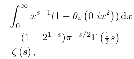
Jacobi%20nome

SearchAdvancedHelp

(0.001 seconds)

21—30 of 215 matching pages

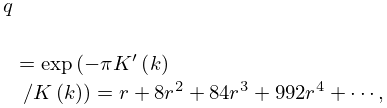
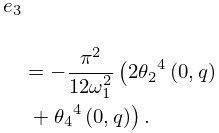
21: 19.5 Maclaurin and Related Expansions

… ► ►For Jacobi’s nome $q$: ►

19.5.5 $$q=\exp \left(-\pi K^{\prime }\left(k\right)/K\left(k\right)\right)=r+8r^2+84r^3+992r^4+\mathrm{\cdots },$$ $r=\frac{1}{16}{k}^2$, $0\le k\le 1$.

ⓘ

Symbols:

$\pi$: the ratio of the circumference of a circle to its diameter, $K^{\prime }\left(k\right)$: Legendre’s complementary complete elliptic integral of the first kind, $K\left(k\right)$: Legendre’s complete elliptic integral of the first kind, $\exp z$: exponential function, $q$: nome and $k$: real or complex modulus

Referenced by:

§19.5

Permalink:

http://dlmf.nist.gov/19.5.E5

Encodings:

pMML, png, TeX

See also:

Annotations for §19.5 and Ch.19

… ►

19.5.6 $$q=\lambda +2{\lambda }^5+15{\lambda }^9+150{\lambda }^{13}+1707{\lambda }^{17}+\mathrm{\cdots },$$ $0\le k\le 1$,

ⓘ

Symbols:

$q$: nome and $k$: real or complex modulus

Referenced by:

§19.5, §19.5

Permalink:

http://dlmf.nist.gov/19.5.E6

Encodings:

pMML, png, TeX

See also:

Annotations for §19.5 and Ch.19

… ►

19.5.8 $$K\left(k\right)=\frac{\pi }{2}{\left(1+2\sum _{n=1}^{\mathrm{\infty }}{q}^{n^2}\right)}^2,$$ ,

ⓘ

Symbols:

$\pi$: the ratio of the circumference of a circle to its diameter, $K\left(k\right)$: Legendre’s complete elliptic integral of the first kind, $q$: nome, $n$: nonnegative integer and $k$: real or complex modulus

Referenced by:

§19.5, §19.5

Permalink:

http://dlmf.nist.gov/19.5.E8

Encodings:

pMML, png, TeX

See also:

Annotations for §19.5 and Ch.19

…

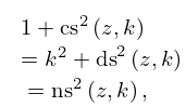
22: 22.6 Elementary Identities

… ►

22.6.2 $$1+{\mathrm{cs}}^2(z,k)=k^2+{\mathrm{ds}}^2(z,k)={\mathrm{ns}}^2(z,k),$$

ⓘ

Symbols:

$\mathrm{cs}(z,k)$: Jacobian elliptic function, $\mathrm{ds}(z,k)$: Jacobian elliptic function, $\mathrm{ns}(z,k)$: Jacobian elliptic function, $z$: complex and $k$: modulus

A&S Ref:

16.9.4

Permalink:

http://dlmf.nist.gov/22.6.E2

Encodings:

pMML, png, TeX

See also:

Annotations for §22.6(i), §22.6 and Ch.22

… ►

22.6.5 $$\mathrm{sn}(2z,k)=\frac{2\mathrm{sn}(z,k)\mathrm{cn}(z,k)\mathrm{dn}(z,k)}{1-k^2{\mathrm{sn}}^4(z,k)},$$

ⓘ

Symbols:

$\mathrm{cn}(z,k)$: Jacobian elliptic function, $\mathrm{dn}(z,k)$: Jacobian elliptic function, $\mathrm{sn}(z,k)$: Jacobian elliptic function, $z$: complex and $k$: modulus

A&S Ref:

16.18.1

Permalink:

http://dlmf.nist.gov/22.6.E5

Encodings:

pMML, png, TeX

See also:

Annotations for §22.6(ii), §22.6 and Ch.22

… ►

22.6.8 $$\mathrm{cd}(2z,k)=\frac{{\mathrm{cd}}^2(z,k)-k_{}^{\prime }{}_{}{}^2{\mathrm{sd}}^2(z,k){\mathrm{nd}}^2(z,k)}{1+k^{2}k_{}^{\prime }{}_{}{}^2{\mathrm{sd}}^4(z,k)},$$

ⓘ

Symbols:

$\mathrm{cd}(z,k)$: Jacobian elliptic function, $\mathrm{nd}(z,k)$: Jacobian elliptic function, $\mathrm{sd}(z,k)$: Jacobian elliptic function, $z$: complex, $k$: modulus and $k^{\prime }$: complementary modulus

Permalink:

http://dlmf.nist.gov/22.6.E8

Encodings:

pMML, png, TeX

See also:

Annotations for §22.6(ii), §22.6 and Ch.22

… ►

§22.6(iv) Rotation of Argument (Jacobi’s Imaginary Transformation)

►

Table 22.6.1: Jacobi’s imaginary transformation of Jacobian elliptic functions.

► ►►

$\mathrm{sn}(\mathrm{i}z,k)$ $=$	$\mathrm{i}\mathrm{sc}(z,k^{\prime })$	$\mathrm{dc}(\mathrm{i}z,k)$ $=$	$\mathrm{dn}(z,k^{\prime })$
…

►

…

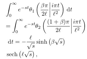
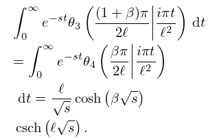
23: 20.10 Integrals

… ►

20.10.1 $${\int }_0^{\mathrm{\infty }}{x}^{s-1}{\theta }_2\left(0\right|\mathrm{i}{x}^2)dx=2^s(1-2^{-s}){\pi }^{-s/2}\mathrm{\Gamma }\left(\frac{1}{2}s\right)\zeta \left(s\right),$$ $\mathrm{\Re }s>1$,

ⓘ

Symbols:

$\mathrm{\Gamma }\left(z\right)$: gamma function, ${\theta }_j\left(z\right|\tau )$: theta function, $\zeta \left(s\right)$: Riemann zeta function, $\pi$: the ratio of the circumference of a circle to its diameter, $dx$: differential of $x$ , $\mathrm{i}$: imaginary unit, $\int$: integral and $\mathrm{\Re }$: real part

Keywords:

Mellin transform

Referenced by:

§20.10(i), Erratum (V1.1.5) for §20.10(i)

Permalink:

http://dlmf.nist.gov/20.10.E1

Encodings:

pMML, png, TeX

Modification (effective with 1.1.5):

Originally the constraint was $\mathrm{\Re }s>2$. This can be relaxed to $\mathrm{\Re }s>1$ because ${\theta }_2\left(0\right|\mathrm{i}{x}^2)=x^{-1}{\theta }_4\left(0\right|\mathrm{i}{x}^{-2})\sim x^{-1}$ as $x\to 0+$, which follows from (20.7.31) and (20.4.5).

See also:

Annotations for §20.10(i), §20.10 and Ch.20

►

20.10.2 $${\int }_0^{\mathrm{\infty }}{x}^{s-1}({\theta }_3\left(0\right|\mathrm{i}{x}^2)-1)dx={\pi }^{-s/2}\mathrm{\Gamma }\left(\frac{1}{2}s\right)\zeta \left(s\right),$$ $\mathrm{\Re }s>1$,

ⓘ

Symbols:

$\mathrm{\Gamma }\left(z\right)$: gamma function, ${\theta }_j\left(z\right|\tau )$: theta function, $\zeta \left(s\right)$: Riemann zeta function, $\pi$: the ratio of the circumference of a circle to its diameter, $dx$: differential of $x$ , $\mathrm{i}$: imaginary unit, $\int$: integral and $\mathrm{\Re }$: real part

Keywords:

Mellin transform

Referenced by:

§20.10(i), Erratum (V1.1.5) for §20.10(i)

Permalink:

http://dlmf.nist.gov/20.10.E2

Encodings:

pMML, png, TeX

Modification (effective with 1.1.5):

Originally the constraint was $\mathrm{\Re }s>2$. This can be relaxed to $\mathrm{\Re }s>1$ because ${\theta }_3\left(0\right|\mathrm{i}{x}^2)=x^{-1}{\theta }_3\left(0\right|\mathrm{i}{x}^{-2})\sim x^{-1}$ as $x\to 0+$, which follows from (20.7.32) and (20.4.4).

See also:

Annotations for §20.10(i), §20.10 and Ch.20

►

20.10.3 $${\int }_0^{\mathrm{\infty }}{x}^{s-1}(1-{\theta }_4\left(0\right|\mathrm{i}{x}^2))dx=(1-2^{1-s}){\pi }^{-s/2}\mathrm{\Gamma }\left(\frac{1}{2}s\right)\zeta \left(s\right),$$ $\mathrm{\Re }s>0$.

ⓘ

Symbols:

$\mathrm{\Gamma }\left(z\right)$: gamma function, ${\theta }_j\left(z\right|\tau )$: theta function, $\zeta \left(s\right)$: Riemann zeta function, $\pi$: the ratio of the circumference of a circle to its diameter, $dx$: differential of $x$ , $\mathrm{i}$: imaginary unit, $\int$: integral and $\mathrm{\Re }$: real part

Keywords:

Mellin transform

Referenced by:

§20.10(i), Erratum (V1.1.5) for §20.10(i)

Permalink:

http://dlmf.nist.gov/20.10.E3

Encodings:

pMML, png, TeX

Modification (effective with 1.1.5):

Originally the constraint was $\mathrm{\Re }s>2$. This can be relaxed to $\mathrm{\Re }s>0$ because $1-{\theta }_4\left(0\right|\mathrm{i}{x}^2)=1-x^{-1}{\theta }_2\left(0\right|\mathrm{i}{x}^{-2})\sim 1$ as $x\to 0+$, which follows from (20.7.33) and (20.4.3).

See also:

Annotations for §20.10(i), §20.10 and Ch.20

… ►

20.10.4 $${\int }_0^{\mathrm{\infty }}{\mathrm{e}}^{-st}{\theta }_1\left(\frac{\beta \pi }{2\mathrm{\ell }}\right|\frac{\mathrm{i}\pi t}{{\mathrm{\ell }}^2})dt={\int }_0^{\mathrm{\infty }}{\mathrm{e}}^{-st}{\theta }_2\left(\frac{(1+\beta )\pi }{2\mathrm{\ell }}\right|\frac{\mathrm{i}\pi t}{{\mathrm{\ell }}^2})dt=-\frac{\mathrm{\ell }}{\sqrt{s}}\sinh \left(\beta \sqrt{s}\right)\mathrm{sech}\left(\mathrm{\ell }\sqrt{s}\right),$$

ⓘ

Symbols:

${\theta }_j\left(z\right|\tau )$: theta function, $\pi$: the ratio of the circumference of a circle to its diameter, $dx$: differential of $x$ , $\mathrm{e}$: base of natural logarithm, $\mathrm{sech}z$: hyperbolic secant function, $\sinh z$: hyperbolic sine function, $\mathrm{i}$: imaginary unit, $\int$: integral, $s$: parameter, $\beta$: parameter and $\mathrm{\ell }$: parameter

Permalink:

http://dlmf.nist.gov/20.10.E4

Encodings:

pMML, png, TeX

See also:

Annotations for §20.10(ii), §20.10 and Ch.20

►

20.10.5 $${\int }_0^{\mathrm{\infty }}{\mathrm{e}}^{-st}{\theta }_3\left(\frac{(1+\beta )\pi }{2\mathrm{\ell }}\right|\frac{\mathrm{i}\pi t}{{\mathrm{\ell }}^2})dt={\int }_0^{\mathrm{\infty }}{\mathrm{e}}^{-st}{\theta }_4\left(\frac{\beta \pi }{2\mathrm{\ell }}\right|\frac{\mathrm{i}\pi t}{{\mathrm{\ell }}^2})dt=\frac{\mathrm{\ell }}{\sqrt{s}}\cosh \left(\beta \sqrt{s}\right)\mathrm{csch}\left(\mathrm{\ell }\sqrt{s}\right).$$

ⓘ

Symbols:

${\theta }_j\left(z\right|\tau )$: theta function, $\pi$: the ratio of the circumference of a circle to its diameter, $dx$: differential of $x$ , $\mathrm{e}$: base of natural logarithm, $\mathrm{csch}z$: hyperbolic cosecant function, $\cosh z$: hyperbolic cosine function, $\mathrm{i}$: imaginary unit, $\int$: integral, $s$: parameter, $\beta$: parameter and $\mathrm{\ell }$: parameter

Permalink:

http://dlmf.nist.gov/20.10.E5

Encodings:

pMML, png, TeX

See also:

Annotations for §20.10(ii), §20.10 and Ch.20

…

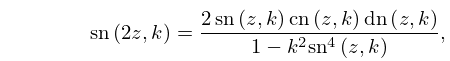
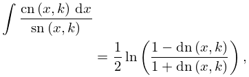
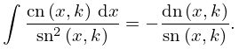
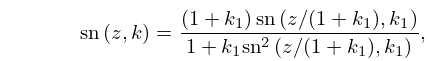
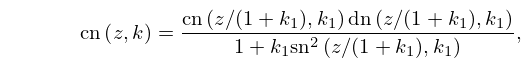
24: 23.6 Relations to Other Functions

… ►

23.6.2 $$e_1=\frac{{\pi }^2}{12{\omega }_1^2}\left({\theta }_2^4(0,q)+2{\theta }_4^4(0,q)\right),$$

ⓘ

Symbols:

${\theta }_j(z,q)$: theta function, $e_j$: Weierstrass lattice roots, $\pi$: the ratio of the circumference of a circle to its diameter, $𝕃$: lattice, $q$: nome and ${\omega }_1$, ${\omega }_3$, ${\omega }_2=-{\omega }_1-{\omega }_3$: lattice generators

A&S Ref:

18.10.12, 18.10.13, 18.10.14, and 18.10.9, 18.10.10, 18.10.11

Referenced by:

§23.22(ii), §23.22(i), §23.6(i), §23.6(ii)

Permalink:

http://dlmf.nist.gov/23.6.E2

Encodings:

pMML, png, TeX

See also:

Annotations for §23.6(i), §23.6 and Ch.23

►

23.6.3 $$e_2=\frac{{\pi }^2}{12{\omega }_1^2}\left({\theta }_2^4(0,q)-{\theta }_4^4(0,q)\right),$$

ⓘ

Symbols:

${\theta }_j(z,q)$: theta function, $e_j$: Weierstrass lattice roots, $\pi$: the ratio of the circumference of a circle to its diameter, $𝕃$: lattice, $q$: nome and ${\omega }_1$, ${\omega }_3$, ${\omega }_2=-{\omega }_1-{\omega }_3$: lattice generators

A&S Ref:

18.10.12, 18.10.13, 18.10.14, and 18.10.9, 18.10.10, 18.10.11

Permalink:

http://dlmf.nist.gov/23.6.E3

Encodings:

pMML, png, TeX

See also:

Annotations for §23.6(i), §23.6 and Ch.23

►

23.6.4 $$e_3=-\frac{{\pi }^2}{12{\omega }_1^2}\left(2{\theta }_2^4(0,q)+{\theta }_4^4(0,q)\right).$$

ⓘ

Symbols:

${\theta }_j(z,q)$: theta function, $e_j$: Weierstrass lattice roots, $\pi$: the ratio of the circumference of a circle to its diameter, $𝕃$: lattice, $q$: nome and ${\omega }_1$, ${\omega }_3$, ${\omega }_2=-{\omega }_1-{\omega }_3$: lattice generators

A&S Ref:

18.10.12, 18.10.13, 18.10.14, and 18.10.9, 18.10.10, 18.10.11

Referenced by:

§23.22(ii), §23.6(ii)

Permalink:

http://dlmf.nist.gov/23.6.E4

Encodings:

pMML, png, TeX

See also:

Annotations for §23.6(i), §23.6 and Ch.23

… ►Similar results for the other nine Jacobi functions can be constructed with the aid of the transformations given by Table 22.4.3. ►For representations of the Jacobi functions $\mathrm{sn}$, $\mathrm{cn}$, and $\mathrm{dn}$ as quotients of $\sigma$-functions see Lawden (1989, §§6.2, 6.3). …

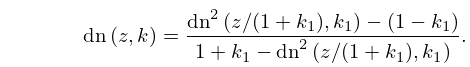
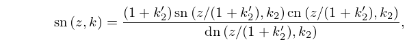
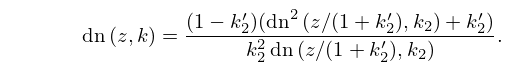
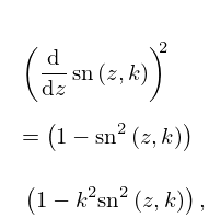
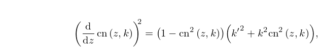
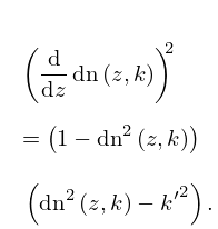
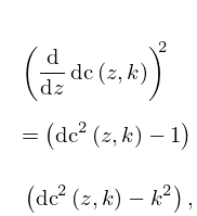
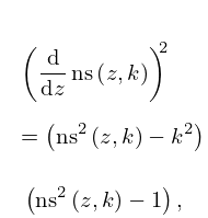
25: 22.13 Derivatives and Differential Equations

… ►

22.13.1 $${\left(\frac{d}{dz}\mathrm{sn}(z,k)\right)}^2=\left(1-{\mathrm{sn}}^2(z,k)\right)\left(1-k^2{\mathrm{sn}}^2(z,k)\right),$$

ⓘ

Symbols:

$\mathrm{sn}(z,k)$: Jacobian elliptic function, $\frac{df}{dx}$: derivative of $f$ with respect to $x$ , $z$: complex and $k$: modulus

Referenced by:

§22.13(iii), §22.18(iv)

Permalink:

http://dlmf.nist.gov/22.13.E1

Encodings:

pMML, png, TeX

See also:

Annotations for §22.13(ii), §22.13 and Ch.22

►

22.13.2 $${\left(\frac{d}{dz}\mathrm{cn}(z,k)\right)}^2=\left(1-{\mathrm{cn}}^2(z,k)\right)\left(k_{}^{\prime }{}_{}{}^2+k^2{\mathrm{cn}}^2(z,k)\right),$$

ⓘ

Symbols:

$\mathrm{cn}(z,k)$: Jacobian elliptic function, $\frac{df}{dx}$: derivative of $f$ with respect to $x$ , $z$: complex, $k$: modulus and $k^{\prime }$: complementary modulus

Permalink:

http://dlmf.nist.gov/22.13.E2

Encodings:

pMML, png, TeX

See also:

Annotations for §22.13(ii), §22.13 and Ch.22

►

22.13.3 $${\left(\frac{d}{dz}\mathrm{dn}(z,k)\right)}^2=\left(1-{\mathrm{dn}}^2(z,k)\right)\left({\mathrm{dn}}^2(z,k)-k_{}^{\prime }{}_{}{}^2\right).$$

ⓘ

Symbols:

$\mathrm{dn}(z,k)$: Jacobian elliptic function, $\frac{df}{dx}$: derivative of $f$ with respect to $x$ , $z$: complex, $k$: modulus and $k^{\prime }$: complementary modulus

Permalink:

http://dlmf.nist.gov/22.13.E3

Encodings:

pMML, png, TeX

See also:

Annotations for §22.13(ii), §22.13 and Ch.22

… ►

22.13.7 $${\left(\frac{d}{dz}\mathrm{dc}(z,k)\right)}^2=\left({\mathrm{dc}}^2(z,k)-1\right)\left({\mathrm{dc}}^2(z,k)-k^2\right),$$

ⓘ

Symbols:

$\mathrm{dc}(z,k)$: Jacobian elliptic function, $\frac{df}{dx}$: derivative of $f$ with respect to $x$ , $z$: complex and $k$: modulus

Permalink:

http://dlmf.nist.gov/22.13.E7

Encodings:

pMML, png, TeX

See also:

Annotations for §22.13(ii), §22.13 and Ch.22

… ►

22.13.10 $${\left(\frac{d}{dz}\mathrm{ns}(z,k)\right)}^2=\left({\mathrm{ns}}^2(z,k)-k^2\right)\left({\mathrm{ns}}^2(z,k)-1\right),$$

ⓘ

Symbols:

$\mathrm{ns}(z,k)$: Jacobian elliptic function, $\frac{df}{dx}$: derivative of $f$ with respect to $x$ , $z$: complex and $k$: modulus

Permalink:

http://dlmf.nist.gov/22.13.E10

Encodings:

pMML, png, TeX

See also:

Annotations for §22.13(ii), §22.13 and Ch.22

…

26: 22.4 Periods, Poles, and Zeros

… ►For example, the poles of $\mathrm{sn}(z,k)$, abbreviated as $\mathrm{sn}$ in the following tables, are at $z=2mK+(2n+1)\mathrm{i}{K}^{\prime }$. … ►Then: (a) In any lattice unit cell $\mathrm{p}\mathrm{q}(z,k)$ has a simple zero at $z=\text{p}$ and a simple pole at $z=\text{q}$. (b) The difference between p and the nearest q is a half-period of $\mathrm{p}\mathrm{q}(z,k)$. This half-period will be plus or minus a member of the triple $K,\mathrm{i}{K}^{\prime },K+\mathrm{i}{K}^{\prime }$; the other two members of this triple are quarter periods of $\mathrm{p}\mathrm{q}(z,k)$. … ►For example, $\mathrm{sn}(z+K,k)=\mathrm{cd}(z,k)$. …

27: 18.7 Interrelations and Limit Relations

… ►

Ultraspherical and Jacobi

… ►

Chebyshev, Ultraspherical, and Jacobi

… ►

Legendre, Ultraspherical, and Jacobi

… ►

Jacobi $\to$ Laguerre

… ►

Jacobi $\to$ Hermite

…

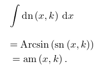
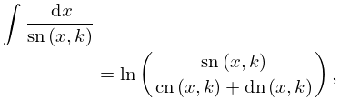
28: 22.14 Integrals

… ►

22.14.3 $$\int \mathrm{dn}(x,k)dx=\mathrm{Arcsin}\left(\mathrm{sn}(x,k)\right)=\mathrm{am}(x,k).$$

ⓘ

Symbols:

$\mathrm{am}(x,k)$: Jacobi’s amplitude function, $\mathrm{dn}(z,k)$: Jacobian elliptic function, $\mathrm{sn}(z,k)$: Jacobian elliptic function, $dx$: differential of $x$ , $\int$: integral, $\mathrm{Arcsin}z$: general arcsine function, $x$: real and $k$: modulus

A&S Ref:

16.24.3

Permalink:

http://dlmf.nist.gov/22.14.E3

Encodings:

pMML, png, TeX

See also:

Annotations for §22.14(i), §22.14 and Ch.22

… ►See §22.16(i) for $\mathrm{am}(z,k)$. … ►

22.14.13 $$\int \frac{dx}{\mathrm{sn}(x,k)}=\ln \left(\frac{\mathrm{sn}(x,k)}{\mathrm{cn}(x,k)+\mathrm{dn}(x,k)}\right),$$

ⓘ

Symbols:

$\mathrm{cn}(z,k)$: Jacobian elliptic function, $\mathrm{dn}(z,k)$: Jacobian elliptic function, $\mathrm{sn}(z,k)$: Jacobian elliptic function, $dx$: differential of $x$ , $\int$: integral, $\ln z$: principal branch of logarithm function, $x$: real and $k$: modulus

Referenced by:

§22.14(iii)

Permalink:

http://dlmf.nist.gov/22.14.E13

Encodings:

pMML, png, TeX

See also:

Annotations for §22.14(iii), §22.14 and Ch.22

►

22.14.14 $$\int \frac{\mathrm{cn}(x,k)dx}{\mathrm{sn}(x,k)}=\frac{1}{2}\ln \left(\frac{1-\mathrm{dn}(x,k)}{1+\mathrm{dn}(x,k)}\right),$$

ⓘ

Symbols:

$\mathrm{cn}(z,k)$: Jacobian elliptic function, $\mathrm{dn}(z,k)$: Jacobian elliptic function, $\mathrm{sn}(z,k)$: Jacobian elliptic function, $dx$: differential of $x$ , $\int$: integral, $\ln z$: principal branch of logarithm function, $x$: real and $k$: modulus

Permalink:

http://dlmf.nist.gov/22.14.E14

Encodings:

pMML, png, TeX

See also:

Annotations for §22.14(iii), §22.14 and Ch.22

►

22.14.15 $$\int \frac{\mathrm{cn}(x,k)dx}{{\mathrm{sn}}^2(x,k)}=-\frac{\mathrm{dn}(x,k)}{\mathrm{sn}(x,k)}.$$

ⓘ

Symbols:

$\mathrm{cn}(z,k)$: Jacobian elliptic function, $\mathrm{dn}(z,k)$: Jacobian elliptic function, $\mathrm{sn}(z,k)$: Jacobian elliptic function, $dx$: differential of $x$ , $\int$: integral, $x$: real and $k$: modulus

Referenced by:

§22.14(iii)

Permalink:

http://dlmf.nist.gov/22.14.E15

Encodings:

pMML, png, TeX

See also:

Annotations for §22.14(iii), §22.14 and Ch.22

…

29: 22.7 Landen Transformations

… ►

22.7.2 $$\mathrm{sn}(z,k)=\frac{(1+k_1)\mathrm{sn}(z/(1+k_1),k_1)}{1+k_1{\mathrm{sn}}^2(z/(1+k_1),k_1)},$$

ⓘ

Symbols:

$\mathrm{sn}(z,k)$: Jacobian elliptic function, $z$: complex, $k$: modulus and $k_1$: change of variable

A&S Ref:

16.12.2

Referenced by:

§22.20(iii)

Permalink:

http://dlmf.nist.gov/22.7.E2

Encodings:

pMML, png, TeX

See also:

Annotations for §22.7(i), §22.7 and Ch.22

►

22.7.3 $$\mathrm{cn}(z,k)=\frac{\mathrm{cn}(z/(1+k_1),k_1)\mathrm{dn}(z/(1+k_1),k_1)}{1+k_1{\mathrm{sn}}^2(z/(1+k_1),k_1)},$$

ⓘ

Symbols:

$\mathrm{cn}(z,k)$: Jacobian elliptic function, $\mathrm{dn}(z,k)$: Jacobian elliptic function, $\mathrm{sn}(z,k)$: Jacobian elliptic function, $z$: complex, $k$: modulus and $k_1$: change of variable

A&S Ref:

16.12.3

Referenced by:

§22.20(iii)

Permalink:

http://dlmf.nist.gov/22.7.E3

Encodings:

pMML, png, TeX

See also:

Annotations for §22.7(i), §22.7 and Ch.22

►

22.7.4 $$\mathrm{dn}(z,k)=\frac{{\mathrm{dn}}^2(z/(1+k_1),k_1)-(1-k_1)}{1+k_1-{\mathrm{dn}}^2(z/(1+k_1),k_1)}.$$

ⓘ

Symbols:

$\mathrm{dn}(z,k)$: Jacobian elliptic function, $z$: complex, $k$: modulus and $k_1$: change of variable

A&S Ref:

16.12.4

Referenced by:

§22.20(iii)

Permalink:

http://dlmf.nist.gov/22.7.E4

Encodings:

pMML, png, TeX

See also:

Annotations for §22.7(i), §22.7 and Ch.22

… ►

22.7.6 $$\mathrm{sn}(z,k)=\frac{(1+k_2^{\prime })\mathrm{sn}(z/(1+k_2^{\prime }),k_2)\mathrm{cn}(z/(1+k_2^{\prime }),k_2)}{\mathrm{dn}(z/(1+k_2^{\prime }),k_2)},$$

ⓘ

Symbols:

$\mathrm{cn}(z,k)$: Jacobian elliptic function, $\mathrm{dn}(z,k)$: Jacobian elliptic function, $\mathrm{sn}(z,k)$: Jacobian elliptic function, $z$: complex, $k$: modulus, $k_2$: change of variable and $k_2^{\prime }$: change of variable

A&S Ref:

16.14.2

Permalink:

http://dlmf.nist.gov/22.7.E6

Encodings:

pMML, png, TeX

See also:

Annotations for §22.7(ii), §22.7 and Ch.22

… ►

22.7.8 $$\mathrm{dn}(z,k)=\frac{(1-k_2^{\prime })({\mathrm{dn}}^2(z/(1+k_2^{\prime }),k_2)+k_2^{\prime })}{k_2^2\mathrm{dn}(z/(1+k_2^{\prime }),k_2)}.$$

ⓘ

Symbols:

$\mathrm{dn}(z,k)$: Jacobian elliptic function, $z$: complex, $k$: modulus, $k_2$: change of variable and $k_2^{\prime }$: change of variable

A&S Ref:

16.14.4

Permalink:

http://dlmf.nist.gov/22.7.E8

Encodings:

pMML, png, TeX

See also:

Annotations for §22.7(ii), §22.7 and Ch.22

…

30: 18.5 Explicit Representations

… ►

§18.5(iii) Finite Power Series, the Hypergeometric Function, and Generalized Hypergeometric Functions

… ►

Jacobi

… ►For corresponding formulas for Chebyshev, Legendre, and the Hermite ${\mathrm{𝐻𝑒}}_n$ polynomials apply (18.7.3)–(18.7.6), (18.7.9), and (18.7.11). … ►The first of each of equations (18.5.7) and (18.5.8) can be regarded as definitions of $P_n^{(\alpha ,\beta )}\left(x\right)$ when the conditions $\alpha >-1$ and $\beta >-1$ are not satisfied. …For this reason, and also in the interest of simplicity, in the case of the Jacobi polynomials $P_n^{(\alpha ,\beta )}\left(x\right)$ we assume throughout this chapter that $\alpha >-1$ and $\beta >-1$, unless stated otherwise. …