Glaisher constant

SearchAdvancedHelp

(0.002 seconds)

31—40 of 441 matching pages

31: 18.25 Wilson Class: Definitions

… ►Table 18.25.1 lists the transformations of variable, orthogonality ranges, and parameter constraints that are needed in §18.2(i) for the Wilson polynomials $W_n(x;a,b,c,d)$, continuous dual Hahn polynomials $S_n(x;a,b,c)$, Racah polynomials $R_n(x;\alpha ,\beta ,\gamma ,\delta )$, and dual Hahn polynomials $R_n(x;\gamma ,\delta ,N)$. … ►

$$\gamma ,\delta >-1,\beta >N+\gamma .$$

►

… ►

►The first four sets imply $\gamma +\delta >-2$, and the last four imply . …

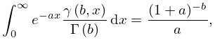
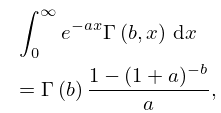
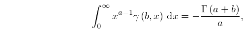
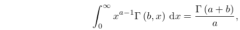
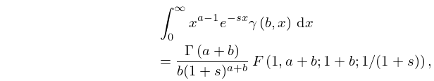
32: 8.14 Integrals

… ►

8.14.1 $${\int }_0^{\mathrm{\infty }}{\mathrm{e}}^{-ax}\frac{\gamma (b,x)}{\mathrm{\Gamma }\left(b\right)}dx=\frac{{(1+a)}^{-b}}{a},$$ $\mathrm{\Re }a>0$, $\mathrm{\Re }b>-1$,

ⓘ

Symbols:

$\mathrm{\Gamma }\left(z\right)$: gamma function, $dx$: differential of $x$ , $\mathrm{e}$: base of natural logarithm, $\gamma (a,z)$: incomplete gamma function, $\int$: integral, $\mathrm{\Re }$: real part, $x$: real variable and $a$: parameter

Referenced by:

§8.14, §8.14

Permalink:

http://dlmf.nist.gov/8.14.E1

Encodings:

pMML, png, TeX

See also:

Annotations for §8.14 and Ch.8

►

8.14.2 $${\int }_0^{\mathrm{\infty }}{\mathrm{e}}^{-ax}\mathrm{\Gamma }(b,x)dx=\mathrm{\Gamma }\left(b\right)\frac{1-{(1+a)}^{-b}}{a},$$ $\mathrm{\Re }a>-1$, $\mathrm{\Re }b>-1$.

ⓘ

Symbols:

$\mathrm{\Gamma }\left(z\right)$: gamma function, $dx$: differential of $x$ , $\mathrm{e}$: base of natural logarithm, $\mathrm{\Gamma }(a,z)$: incomplete gamma function, $\int$: integral, $\mathrm{\Re }$: real part, $x$: real variable and $a$: parameter

A&S Ref:

6.5.36

Referenced by:

§8.14, §8.14

Permalink:

http://dlmf.nist.gov/8.14.E2

Encodings:

pMML, png, TeX

See also:

Annotations for §8.14 and Ch.8

… ►

8.14.3 $${\int }_0^{\mathrm{\infty }}{x}^{a-1}\gamma (b,x)dx=-\frac{\mathrm{\Gamma }\left(a+b\right)}{a},$$ , $\mathrm{\Re }\left(a+b\right)>0$,

ⓘ

Symbols:

$\mathrm{\Gamma }\left(z\right)$: gamma function, $dx$: differential of $x$ , $\gamma (a,z)$: incomplete gamma function, $\int$: integral, $\mathrm{\Re }$: real part, $x$: real variable and $a$: parameter

Referenced by:

§8.14

Permalink:

http://dlmf.nist.gov/8.14.E3

Encodings:

pMML, png, TeX

See also:

Annotations for §8.14 and Ch.8

►

8.14.4 $${\int }_0^{\mathrm{\infty }}{x}^{a-1}\mathrm{\Gamma }(b,x)dx=\frac{\mathrm{\Gamma }\left(a+b\right)}{a},$$ $\mathrm{\Re }a>0$, $\mathrm{\Re }\left(a+b\right)>0$,

ⓘ

Symbols:

$\mathrm{\Gamma }\left(z\right)$: gamma function, $dx$: differential of $x$ , $\mathrm{\Gamma }(a,z)$: incomplete gamma function, $\int$: integral, $\mathrm{\Re }$: real part, $x$: real variable and $a$: parameter

A&S Ref:

6.5.37

Permalink:

http://dlmf.nist.gov/8.14.E4

Encodings:

pMML, png, TeX

See also:

Annotations for §8.14 and Ch.8

►

8.14.5 $${\int }_0^{\mathrm{\infty }}{x}^{a-1}{\mathrm{e}}^{-sx}\gamma (b,x)dx=\frac{\mathrm{\Gamma }\left(a+b\right)}{b{(1+s)}^{a+b}}F(1,a+b;1+b;1/(1+s)),$$ $\mathrm{\Re }s>0$, $\mathrm{\Re }\left(a+b\right)>0$,

ⓘ

Symbols:

$\mathrm{\Gamma }\left(z\right)$: gamma function, $F(a,b;c;z)$ or $F(\genfrac{}{}{0pt}{}{a,b}{c};z)$: $={}_2{}^{}F_1^{}(a,b;c;z)$ Gauss’ hypergeometric function, $dx$: differential of $x$ , $\mathrm{e}$: base of natural logarithm, $\gamma (a,z)$: incomplete gamma function, $\int$: integral, $\mathrm{\Re }$: real part, $x$: real variable and $a$: parameter

Permalink:

http://dlmf.nist.gov/8.14.E5

Encodings:

pMML, png, TeX

See also:

Annotations for §8.14 and Ch.8

…

33: 30.16 Methods of Computation

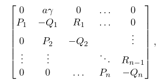
… ►For $m=2$, $n=4$, ${\gamma }^2=10$, … ►If $|{\gamma }^2|$ is large, then we can use the asymptotic expansions referred to in §30.9 to approximate ${\mathrm{𝖯𝗌}}_n^m(x,{\gamma }^2)$. … ►If ${\lambda }_n^m\left({\gamma }^2\right)$ is known, then ${\mathrm{𝖯𝗌}}_n^m(x,{\gamma }^2)$ can be found by summing (30.8.1). The coefficients $a_{n,r}^m({\gamma }^2)$ are computed as the recessive solution of (30.8.4) (§3.6), and normalized via (30.8.5). … ►The coefficients $a_{n,k}^m({\gamma }^2)$ calculated in §30.16(ii) can be used to compute $S_n^{m(j)}(z,\gamma )$, $j=1,2,3,4$ from (30.11.3) as well as the connection coefficients $K_n^m(\gamma )$ from (30.11.10) and (30.11.11). …

34: 4.34 Derivatives and Differential Equations

… ►

4.34.11 $$w=A\cosh \left(az\right)+B\sinh \left(az\right),$$

ⓘ

Symbols:

$\cosh z$: hyperbolic cosine function, $\sinh z$: hyperbolic sine function, $a$: real or complex constant, $z$: complex variable, $w$: solution, $A$: arbitrary constant and $B$: arbitrary constant

Permalink:

http://dlmf.nist.gov/4.34.E11

Encodings:

pMML, png, TeX

See also:

Annotations for §4.34 and Ch.4

►

4.34.12 $$w=(1/a)\sinh \left(az+c\right),$$

ⓘ

Symbols:

$\sinh z$: hyperbolic sine function, $a$: real or complex constant, $z$: complex variable, $w$: solution and $c$: arbitrary constant

Permalink:

http://dlmf.nist.gov/4.34.E12

Encodings:

pMML, png, TeX

See also:

Annotations for §4.34 and Ch.4

►

4.34.13 $$w=(1/a)\cosh \left(az+c\right),$$

ⓘ

Symbols:

$\cosh z$: hyperbolic cosine function, $a$: real or complex constant, $z$: complex variable, $w$: solution and $c$: arbitrary constant

Permalink:

http://dlmf.nist.gov/4.34.E13

Encodings:

pMML, png, TeX

See also:

Annotations for §4.34 and Ch.4

►

4.34.14 $$w=(1/a)\coth \left(az+c\right),$$

ⓘ

Symbols:

$\coth z$: hyperbolic cotangent function, $a$: real or complex constant, $z$: complex variable, $w$: solution and $c$: arbitrary constant

Permalink:

http://dlmf.nist.gov/4.34.E14

Encodings:

pMML, png, TeX

See also:

Annotations for §4.34 and Ch.4

►where $A,B,c$ are arbitrary constants. …

35: 8.13 Zeros

… ►

§8.13(i) $x$-Zeros of ${\gamma }^{\ast }(a,x)$

►The function ${\gamma }^{\ast }(a,x)$ has no real zeros for $a\ge 0$. … ►

§8.13(ii) $\lambda$-Zeros of $\gamma (a,\lambda a)$ and $\mathrm{\Gamma }(a,\lambda a)$

►For information on the distribution and computation of zeros of $\gamma (a,\lambda a)$ and $\mathrm{\Gamma }(a,\lambda a)$ in the complex $\lambda$-plane for large values of the positive real parameter $a$ see Temme (1995a). ►

§8.13(iii) $a$-Zeros of ${\gamma }^{\ast }(a,x)$

…

36: 30.2 Differential Equations

… ►The equation contains three real parameters $\lambda$, ${\gamma }^2$, and $\mu$. In applications involving prolate spheroidal coordinates ${\gamma }^2$ is positive, in applications involving oblate spheroidal coordinates ${\gamma }^2$ is negative; see §§30.13, 30.14. … ►With $\zeta =\gamma z$ Equation (30.2.1) changes to … ►If $\gamma =0$, Equation (30.2.1) is the associated Legendre differential equation; see (14.2.2). …If $\gamma =0$, Equation (30.2.4) is satisfied by spherical Bessel functions; see (10.47.1).

37: 30.17 Tables

… ►

Stratton et al. (1956) tabulates quantities closely related to ${\lambda }_n^m\left({\gamma }^2\right)$ and $a_{n,k}^m({\gamma }^2)$ for $0\le m\le 8$, $m\le n\le 8$, $-64\le {\gamma }^2\le 64$. Precision is 7S.

… ►

Hanish et al. (1970) gives ${\lambda }_n^m\left({\gamma }^2\right)$ and $S_n^{m(j)}(z,\gamma )$, $j=1,2$, and their first derivatives, for $0\le m\le 2$, $m\le n\le m+49$, $-1600\le {\gamma }^2\le 1600$. The range of $z$ is given by $1\le z\le 10$ if ${\gamma }^2>0$, or $z=-\mathrm{i}\xi$, $0\le \xi \le 2$ if . Precision is 18S.

►

EraŠevskaja et al. (1973, 1976) gives $S^{m(j)}(\mathrm{i}y,-\mathrm{i}c)$, $S^{m(j)}(z,\gamma )$ and their first derivatives for $j=1,2$, $0.5\le c\le 8$, $y=0,0.5,1,1.5$, $0.5\le \gamma \le 8$, $z=1.01,1.1,1.4,1.8$. Precision is 15S.

►

Van Buren et al. (1975) gives ${\lambda }_n^0\left({\gamma }^2\right)$, ${\mathrm{𝖯𝗌}}_n^0(x,{\gamma }^2)$ for $0\le n\le 49$, $-1600\le {\gamma }^2\le 1600$, $-1\le x\le 1$. Precision is 8S.

…

38: 30.11 Radial Spheroidal Wave Functions

… ►Then solutions of (30.2.1) with $\mu =m$ and $\lambda ={\lambda }_n^m\left({\gamma }^2\right)$ are given by …Here $a_{n,k}^{-m}({\gamma }^2)$ is defined by (30.8.2) and (30.8.6), and … ►For fixed $\gamma$, as $z\to \mathrm{\infty }$ in the sector $|\mathrm{ph}z|\le \pi -\delta$ (), … ►

30.11.8 $$S_n^{m(1)}(z,\gamma )=K_n^m(\gamma ){\mathrm{𝑃𝑠}}_n^m(z,{\gamma }^2),$$

ⓘ

Symbols:

$S_n^{m(j)}(z,\gamma )$: radial spheroidal wave function, ${\mathrm{𝑃𝑠}}_n^m(z,{\gamma }^2)$: spheroidal wave function of complex argument, $z$: complex variable, $m$: nonnegative integer, $n\ge m$: integer degree, $K_n^m(\gamma )$: connection coefficient and ${\gamma }^2$: real parameter

A&S Ref:

21.10.1 (in different form)

Permalink:

http://dlmf.nist.gov/30.11.E8

Encodings:

pMML, png, TeX

See also:

Annotations for §30.11(v), §30.11 and Ch.30

… ►where …

39: 5.4 Special Values and Extrema

… ►

$\mathrm{\Gamma }\left(1\right)=1,$

►

$n!=\mathrm{\Gamma }\left(n+1\right).$

… ►

5.4.11 $${\mathrm{\Gamma }}^{\prime }\left(1\right)=-\gamma .$$

ⓘ

Symbols:

$\mathrm{\Gamma }\left(z\right)$: gamma function and $\gamma$: Euler’s constant

A&S Ref:

6.3.2

Referenced by:

§5.4(i)

Permalink:

http://dlmf.nist.gov/5.4.E11

Encodings:

pMML, png, TeX

See also:

Annotations for §5.4(i), §5.4 and Ch.5

… ►

$\psi \left(1\right)=-\gamma ,$

… ►

5.4.14 $$\psi \left(n+1\right)=\sum _{k=1}^n\frac{1}{k}-\gamma ,$$

ⓘ

Symbols:

$\gamma$: Euler’s constant, $\psi \left(z\right)$: psi (or digamma) function, $n$: nonnegative integer and $k$: nonnegative integer

A&S Ref:

6.3.2

Permalink:

http://dlmf.nist.gov/5.4.E14

Encodings:

pMML, png, TeX

See also:

Annotations for §5.4(ii), §5.4 and Ch.5

…

40: 31.5 Solutions Analytic at Three Singularities: Heun Polynomials

… ►

31.5.1

ⓘ

Symbols:

$\gamma$: real or complex parameter, $n$: nonnegative integer, $a$: complex parameter, $P_j$: coefficient, $Q_j$: coefficient and $R_j$: coefficient

Permalink:

http://dlmf.nist.gov/31.5.E1

Encodings:

pMML, png, TeX

See also:

Annotations for §31.5 and Ch.31

… ►

31.5.2 $${\mathrm{𝐻𝑝}}_{n,m}(a,q_{n,m};-n,\beta ,\gamma ,\delta ;z)=H\mathrm{\ell }(a,q_{n,m};-n,\beta ,\gamma ,\delta ;z)$$

ⓘ

Defines:

${\mathrm{𝐻𝑝}}_{n,m}(a,q_{n,m};-n,\beta ,\gamma ,\delta ;z)$: Heun polynomials

Symbols:

$H\mathrm{\ell }(a,q;\alpha ,\beta ,\gamma ,\delta ;z)$: Heun functions, $z$: complex variable, $\gamma$: real or complex parameter, $\delta$: real or complex parameter, $m$: nonnegative integer, $n$: nonnegative integer, $a$: complex parameter, $q$: real or complex parameter and $\beta$: real or complex parameter

Permalink:

http://dlmf.nist.gov/31.5.E2

Encodings:

pMML, png, TeX

See also:

Annotations for §31.5 and Ch.31

…