Gegenbauer polynomials
(0.002 seconds)
11—20 of 27 matching pages
11: 18.5 Explicit Representations
…
►
…
►
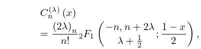
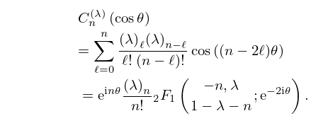
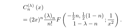
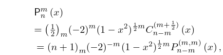
18.5.9
►
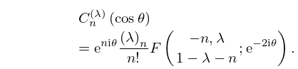
18.5.10
►
18.5.11
…
►Similarly in the cases of the ultraspherical polynomials
and the Laguerre polynomials
we assume that , and , unless
stated otherwise.
…
12: 1.10 Functions of a Complex Variable
…
►
1.10.28
.
…
►
1.10.29
►and hence , that is (18.9.19).
The recurrence relation for in §18.9(i) follows from , and the contour integral representation for in §18.10(iii) is just (1.10.27).
13: 10.23 Sums
14: 18.3 Definitions
…
►
…
15: 15.9 Relations to Other Functions
…
►
Gegenbauer (or Ultraspherical)
►
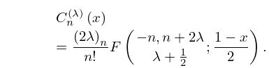
15.9.2
►
15.9.3
►
15.9.4
…
►This is a generalization of Gegenbauer (or ultraspherical) polynomials (§18.3).
…
16: 18.11 Relations to Other Functions
…
►
18.11.1
.
…
17: 18.35 Pollaczek Polynomials
…
►
18.35.8
…
►For the ultraspherical polynomials
, the Meixner–Pollaczek polynomials
and the associated Meixner–Pollaczek polynomials
see §§18.3, 18.19 and 18.30(v), respectively.
…
18: 18.15 Asymptotic Approximations
…
►
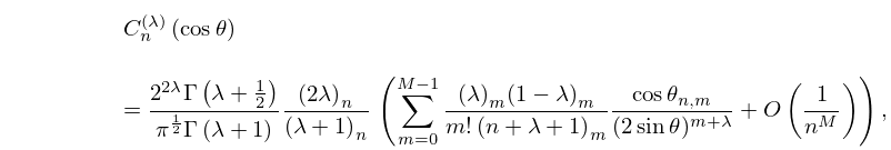
18.15.10
…
►Asymptotic expansions for can be obtained from the results given in §18.15(i) by setting and referring to (18.7.1).
…
19: 10.60 Sums
…
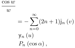
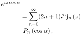
►Then with again denoting the Legendre polynomial of degree ,
►
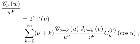
10.60.1
.
►
10.60.2
…
►
10.60.7
►
10.60.8
…
