Gauss sum
(0.003 seconds)
11—20 of 68 matching pages
11: 15.16 Products
12: 16.10 Expansions in Series of Functions
…
►
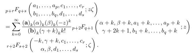
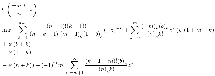
16.10.1
…
►
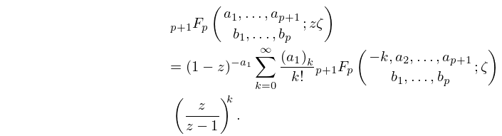
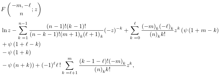
16.10.2
…
►Expansions of the form are discussed in Miller (1997), and further series of generalized hypergeometric functions are given in Luke (1969b, Chapter 9), Luke (1975, §§5.10.2 and 5.11), and Prudnikov et al. (1990, §§5.3, 6.8–6.9).
13: 15.12 Asymptotic Approximations
14: Errata
…
►
Equation (18.38.3)
…
►
Subsection 17.7(iii)
…
18.38.3
, ,
This equation was updated to include the value of the sum in terms of the function. Also the constraint was previously , .
The title of the paragraph which was previously “Andrews’ Terminating -Analog of (17.7.8)” has been changed to “Andrews’ -Analog of the Terminating Version of Watson’s Sum (16.4.6)”. The title of the paragraph which was previously “Andrews’ Terminating -Analog” has been changed to “Andrews’ -Analog of the Terminating Version of Whipple’s Sum (16.4.7)”.
15: 13.14 Definitions and Basic Properties
…
►
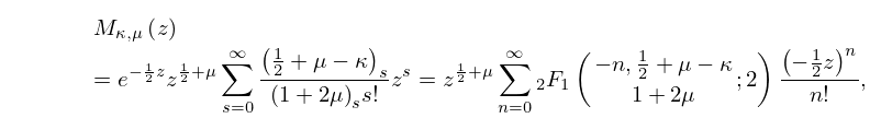
13.14.6
,
…
16: 16.14 Partial Differential Equations
…
►In addition to the four Appell functions there are other sums of double series that cannot be expressed as a product of two functions, and which satisfy pairs of linear partial differential equations of the second order.
…
17: 35.10 Methods of Computation
…
►For small values of the zonal polynomial expansion given by (35.8.1) can be summed numerically.
…
►See Yan (1992) for the and functions of matrix argument in the case , and Bingham et al. (1992) for Monte Carlo simulation on applied to a generalization of the integral (35.5.8).
…
18: 27.2 Functions
…
►It can be expressed as a sum over all primes :
…
►Gauss and Legendre conjectured that is asymptotic to as :
…(See Gauss (1863, Band II, pp. 437–477) and Legendre (1808, p. 394).)
…
►the sum of the th powers of the positive integers that are relatively prime to .
…
►is the sum of the th powers of the divisors of , where the exponent can be real or complex.
…
