Gauss%20multiplication%20formula
(0.002 seconds)
11—20 of 413 matching pages
11: 15.10 Hypergeometric Differential Equation
…
►
…
►(b) If equals , and , then fundamental solutions in the neighborhood of are given by and
►
15.10.8
,
…
►
§15.10(ii) Kummer’s 24 Solutions and Connection Formulas
… ►The connection formulas for the principal branches of Kummer’s solutions are: …12: 15.2 Definitions and Analytical Properties
…
►
§15.2(i) Gauss Series
►The hypergeometric function is defined by the Gauss series … ►On the circle of convergence, , the Gauss series: … ►The same properties hold for , except that as a function of , in general has poles at . … ►Formula (15.4.6) reads . …13: 18.5 Explicit Representations
…
►
§18.5(ii) Rodrigues Formulas
… ►Related formula: …See (Erdélyi et al., 1953b, §10.9(37)) for a related formula for ultraspherical polynomials. … ►For the definitions of , , and see §16.2. … ►and two similar formulas by symmetry; compare the second row in Table 18.6.1. …14: Bibliography
…
►
Exact linearization of a Painlevé transcendent.
Phys. Rev. Lett. 38 (20), pp. 1103–1106.
…
►
On the degrees of irreducible factors of higher order Bernoulli polynomials.
Acta Arith. 62 (4), pp. 329–342.
…
►
Application of the combined nonlinear-condensation transformation to problems in statistical analysis and theoretical physics.
Comput. Phys. Comm. 150 (1), pp. 1–20.
…
►
Gauss, Landen, Ramanujan, the arithmetic-geometric mean, ellipses, , and the Ladies Diary.
Amer. Math. Monthly 95 (7), pp. 585–608.
…
►
Repeated integrals and derivatives of Bessel functions.
SIAM J. Math. Anal. 20 (1), pp. 169–175.
…
15: Errata
…
►
Subsection 17.7(iii)
…
►
Subsections 15.4(i), 15.4(ii)
…
►
Subsection 15.19(v)
…
►
Chapters 8, 20, 36
…
►
References
…
The title of the paragraph which was previously “Andrews’ Terminating -Analog of (17.7.8)” has been changed to “Andrews’ -Analog of the Terminating Version of Watson’s Sum (16.4.6)”. The title of the paragraph which was previously “Andrews’ Terminating -Analog” has been changed to “Andrews’ -Analog of the Terminating Version of Whipple’s Sum (16.4.7)”.
Sentences were added specifying that some equations in these subsections require special care under certain circumstances. Also, (15.4.6) was expanded by adding the formula .
Report by Louis Klauder on 2017-01-01.
A new Subsection Continued Fractions, has been added to cover computation of the Gauss hypergeometric functions by continued fractions.
16: 5.5 Functional Relations
…
►
§5.5(ii) Reflection
… ►§5.5(iii) Multiplication
►Duplication Formula
… ►Gauss’s Multiplication Formula
… ►
5.5.7
…
17: 35.10 Methods of Computation
…
►Other methods include numerical quadrature applied to double and multiple integral representations.
See Yan (1992) for the and functions of matrix argument in the case , and Bingham et al. (1992) for Monte Carlo simulation on applied to a generalization of the integral (35.5.8).
…
18: Bibliography C
…
►
Asymptotic estimates for generalized Stirling numbers.
Analysis (Munich) 20 (1), pp. 1–13.
…
►
Validated computation of certain hypergeometric functions.
ACM Trans. Math. Software 38 (2), pp. Art. 11, 20.
…
►
Coulomb effects in the Klein-Gordon equation for pions.
Phys. Rev. C 20 (2), pp. 696–704.
…
►
The arithmetic-geometric mean of Gauss.
Enseign. Math. (2) 30 (3-4), pp. 275–330.
►
Gauss and the arithmetic-geometric mean.
Notices Amer. Math. Soc. 32 (2), pp. 147–151.
…
19: 16.3 Derivatives and Contiguous Functions
…
►
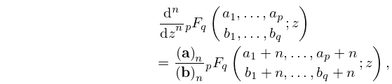
§16.3(i) Differentiation Formulas
►
16.3.1
…
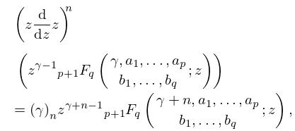
►
16.3.3
…
►Two generalized hypergeometric functions are (generalized)
contiguous if they have the same pair of values of and , and corresponding parameters differ by integers.
…
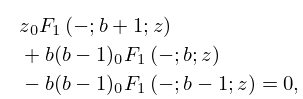
►
16.3.6
…
20: Gergő Nemes
…
►As of September 20, 2021, Nemes performed a complete analysis and acted as main consultant for the update of the source citation and proof metadata for every formula in Chapter 25 Zeta and Related Functions.
…
