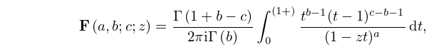
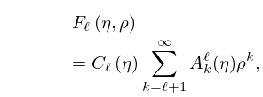
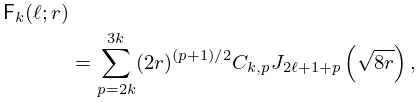
The Olver hypergeometric function , previously omitted
from the left-hand side to make the formula more concise, has been added.
The constraint , originally mentioned in the text, has been
directly added to the formula.
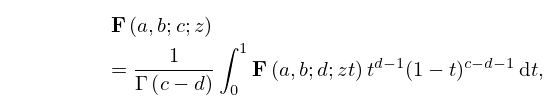
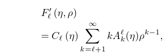
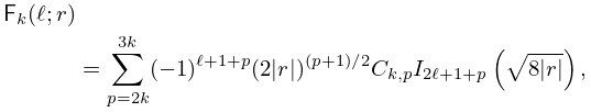
The Olver hypergeometric function , previously omitted
from the left-hand side to make the formula more concise, has been added.
The constraint , originally mentioned in the text, has been
directly added to the formula.
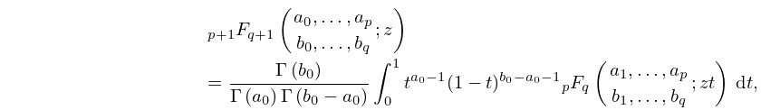
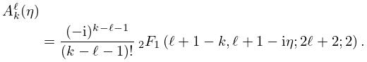
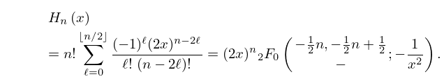
The Olver hypergeometric function , previously omitted
from the left-hand side to make the formula more concise, has been added.
The constraint , originally mentioned in the text, has been
directly added to the formula.
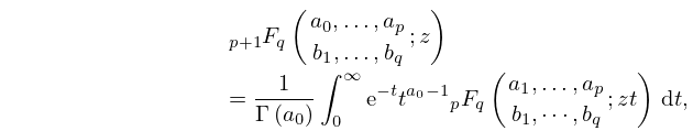
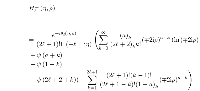
The Olver hypergeometric function , previously omitted
from the left-hand side to make the formula more concise, has been added.
The constraint , originally mentioned in the text, has been
directly added to the formula.
…
►§33.8 supplies continued fractions for and .
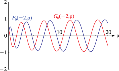
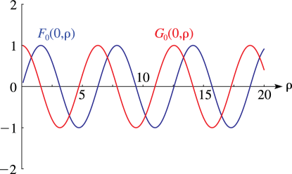
Combined with the Wronskians (33.2.12), the values of , , and their derivatives can be extracted.
…
►Bardin et al. (1972) describes ten different methods for the calculation of and , valid in different regions of the ()-plane.
…
►Hull and Breit (1959) and Barnett (1981b) give WKBJ approximations for and in the region inside the turning point: .
…
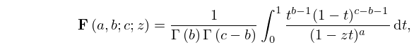
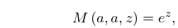
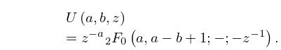
►In this event, the formal power-series expansion of the left-hand side (obtained from (16.2.1)) is the asymptotic expansion of the right-hand side as in the sector , where is an arbitrary small positive constant.
…
►
…
►Laplace transforms and inverse Laplace transforms of generalized hypergeometric functions are given in Prudnikov et al. (1992a, §3.38) and Prudnikov et al. (1992b, §3.36).
…
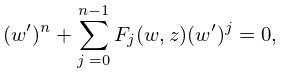
►where is polynomial in with coefficients that are rational functions of .
…
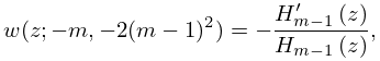
►Solutions for other values of are derived from by application of the Bäcklund transformations (32.7.1) and (32.7.2).
…
►
…
►In (18.5.4_5) see §26.11 for the Fibonacci numbers .
…
►In this equation is as in Table 18.3.1, (reproduced in Table 18.5.1), and , are as in Table 18.5.1.
…
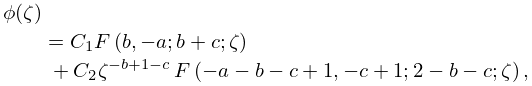
►For the definitions of , , and see §16.2.
…
►
 ►
►
 ►
►
