Euler constant

SearchAdvancedHelp

(0.013 seconds)

21—30 of 339 matching pages

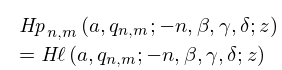
21: 8.13 Zeros

… ►

§8.13(i) $x$-Zeros of ${\gamma }^{\ast }(a,x)$

►The function ${\gamma }^{\ast }(a,x)$ has no real zeros for $a\ge 0$. … ►

§8.13(ii) $\lambda$-Zeros of $\gamma (a,\lambda a)$ and $\mathrm{\Gamma }(a,\lambda a)$

►For information on the distribution and computation of zeros of $\gamma (a,\lambda a)$ and $\mathrm{\Gamma }(a,\lambda a)$ in the complex $\lambda$-plane for large values of the positive real parameter $a$ see Temme (1995a). ►

§8.13(iii) $a$-Zeros of ${\gamma }^{\ast }(a,x)$

…

22: 30.2 Differential Equations

… ►The equation contains three real parameters $\lambda$, ${\gamma }^2$, and $\mu$. In applications involving prolate spheroidal coordinates ${\gamma }^2$ is positive, in applications involving oblate spheroidal coordinates ${\gamma }^2$ is negative; see §§30.13, 30.14. … ►With $\zeta =\gamma z$ Equation (30.2.1) changes to … ►If $\gamma =0$, Equation (30.2.1) is the associated Legendre differential equation; see (14.2.2). …If $\gamma =0$, Equation (30.2.4) is satisfied by spherical Bessel functions; see (10.47.1).

23: 30.17 Tables

… ►

Stratton et al. (1956) tabulates quantities closely related to ${\lambda }_n^m\left({\gamma }^2\right)$ and $a_{n,k}^m({\gamma }^2)$ for $0\le m\le 8$, $m\le n\le 8$, $-64\le {\gamma }^2\le 64$. Precision is 7S.

… ►

Hanish et al. (1970) gives ${\lambda }_n^m\left({\gamma }^2\right)$ and $S_n^{m(j)}(z,\gamma )$, $j=1,2$, and their first derivatives, for $0\le m\le 2$, $m\le n\le m+49$, $-1600\le {\gamma }^2\le 1600$. The range of $z$ is given by $1\le z\le 10$ if ${\gamma }^2>0$, or $z=-\mathrm{i}\xi$, $0\le \xi \le 2$ if . Precision is 18S.

►

EraŠevskaja et al. (1973, 1976) gives $S^{m(j)}(\mathrm{i}y,-\mathrm{i}c)$, $S^{m(j)}(z,\gamma )$ and their first derivatives for $j=1,2$, $0.5\le c\le 8$, $y=0,0.5,1,1.5$, $0.5\le \gamma \le 8$, $z=1.01,1.1,1.4,1.8$. Precision is 15S.

►

Van Buren et al. (1975) gives ${\lambda }_n^0\left({\gamma }^2\right)$, ${\mathrm{𝖯𝗌}}_n^0(x,{\gamma }^2)$ for $0\le n\le 49$, $-1600\le {\gamma }^2\le 1600$, $-1\le x\le 1$. Precision is 8S.

…

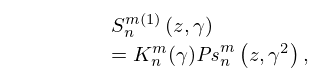
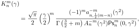
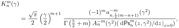
24: 30.11 Radial Spheroidal Wave Functions

… ►Here $a_{n,k}^{-m}({\gamma }^2)$ is defined by (30.8.2) and (30.8.6), and … ►

30.11.8 $$S_n^{m(1)}(z,\gamma )=K_n^m(\gamma ){\mathrm{𝑃𝑠}}_n^m(z,{\gamma }^2),$$

ⓘ

Symbols:

$S_n^{m(j)}(z,\gamma )$: radial spheroidal wave function, ${\mathrm{𝑃𝑠}}_n^m(z,{\gamma }^2)$: spheroidal wave function of complex argument, $z$: complex variable, $m$: nonnegative integer, $n\ge m$: integer degree, $K_n^m(\gamma )$: connection coefficient and ${\gamma }^2$: real parameter

A&S Ref:

21.10.1 (in different form)

Permalink:

http://dlmf.nist.gov/30.11.E8

Encodings:

pMML, png, TeX

See also:

Annotations for §30.11(v), §30.11 and Ch.30

… ►where ►

30.11.10 $$K_n^m(\gamma )=\frac{\sqrt{\pi }}{2}{\left(\frac{\gamma }{2}\right)}^m\frac{{(-1)}^m{a}_{n,\frac{1}{2}(m-n)}^{-m}({\gamma }^2)}{\mathrm{\Gamma }\left(\frac{3}{2}+m\right)A_n^{-m}({\gamma }^2){\mathrm{𝖯𝗌}}_n^m(0,{\gamma }^2)},$$ $n-m$ even,

ⓘ

Symbols:

$\mathrm{\Gamma }\left(z\right)$: gamma function, $\pi$: the ratio of the circumference of a circle to its diameter, ${\mathrm{𝖯𝗌}}_n^m(x,{\gamma }^2)$: spheroidal wave function of the first kind, $m$: nonnegative integer, $n\ge m$: integer degree, $A_n^m({\gamma }^2)$ , $K_n^m(\gamma )$: connection coefficient, ${\gamma }^2$: real parameter and $a_{n,k}^m({\gamma }^2)$: coefficients

Referenced by:

§30.16(iii)

Permalink:

http://dlmf.nist.gov/30.11.E10

Encodings:

pMML, png, TeX

See also:

Annotations for §30.11(v), §30.11 and Ch.30

… ►

30.11.11 $$K_n^m(\gamma )=\frac{\sqrt{\pi }}{2}{\left(\frac{\gamma }{2}\right)}^{m+1}\frac{{(-1)}^m{a}_{n,\frac{1}{2}(m-n+1)}^{-m}({\gamma }^2)}{\mathrm{\Gamma }\left(\frac{5}{2}+m\right)A_n^{-m}({\gamma }^2)({d{\mathrm{𝖯𝗌}}_n^m(z,{\gamma }^2)/dz|}_{z=0})},$$ $n-m$ odd.

ⓘ

Symbols:

$\mathrm{\Gamma }\left(z\right)$: gamma function, $\pi$: the ratio of the circumference of a circle to its diameter, $\frac{df}{dx}$: derivative of $f$ with respect to $x$ , ${\mathrm{𝖯𝗌}}_n^m(x,{\gamma }^2)$: spheroidal wave function of the first kind, $z$: complex variable, $m$: nonnegative integer, $n\ge m$: integer degree, $A_n^m({\gamma }^2)$ , $K_n^m(\gamma )$: connection coefficient, ${\gamma }^2$: real parameter and $a_{n,k}^m({\gamma }^2)$: coefficients

Referenced by:

§30.16(iii)

Permalink:

http://dlmf.nist.gov/30.11.E11

Encodings:

pMML, png, TeX

See also:

Annotations for §30.11(v), §30.11 and Ch.30

…

25: 31.5 Solutions Analytic at Three Singularities: Heun Polynomials

… ►

31.5.1

ⓘ

Symbols:

$\gamma$: real or complex parameter, $n$: nonnegative integer, $a$: complex parameter, $P_j$: coefficient, $Q_j$: coefficient and $R_j$: coefficient

Permalink:

http://dlmf.nist.gov/31.5.E1

Encodings:

pMML, png, TeX

See also:

Annotations for §31.5 and Ch.31

… ►

31.5.2 $${\mathrm{𝐻𝑝}}_{n,m}(a,q_{n,m};-n,\beta ,\gamma ,\delta ;z)=H\mathrm{\ell }(a,q_{n,m};-n,\beta ,\gamma ,\delta ;z)$$

ⓘ

Defines:

${\mathrm{𝐻𝑝}}_{n,m}(a,q_{n,m};-n,\beta ,\gamma ,\delta ;z)$: Heun polynomials

Symbols:

$H\mathrm{\ell }(a,q;\alpha ,\beta ,\gamma ,\delta ;z)$: Heun functions, $z$: complex variable, $\gamma$: real or complex parameter, $\delta$: real or complex parameter, $m$: nonnegative integer, $n$: nonnegative integer, $a$: complex parameter, $q$: real or complex parameter and $\beta$: real or complex parameter

Permalink:

http://dlmf.nist.gov/31.5.E2

Encodings:

pMML, png, TeX

See also:

Annotations for §31.5 and Ch.31

…

26: 31.3 Basic Solutions

… ►

31.3.2 $$a\gamma c_1-q{c}_0=0,$$

ⓘ

Symbols:

$\gamma$: real or complex parameter, $a$: complex parameter, $q$: real or complex parameter and $c_j$: coefficients

Permalink:

http://dlmf.nist.gov/31.3.E2

Encodings:

pMML, png, TeX

See also:

Annotations for §31.3(i), §31.3 and Ch.31

… ►

$$R_j=a(j+1)(j+\gamma ).$$

►Similarly, if $\gamma \ne 1,2,3,\mathrm{\dots }$, then the solution of (31.2.1) that corresponds to the exponent $1-\gamma$ at $z=0$ is ►

31.3.5 $$z^{1-\gamma }H\mathrm{\ell }(a,(a\delta +ϵ)(1-\gamma )+q;\alpha +1-\gamma ,\beta +1-\gamma ,2-\gamma ,\delta ;z).$$

ⓘ

Symbols:

$H\mathrm{\ell }(a,q;\alpha ,\beta ,\gamma ,\delta ;z)$: Heun functions, $z$: complex variable, $\gamma$: real or complex parameter, $\delta$: real or complex parameter, $ϵ$: real or complex parameter, $a$: complex parameter, $q$: real or complex parameter, $\alpha$: real or complex parameter and $\beta$: real or complex parameter

Referenced by:

§31.3(iii), §31.7(ii)

Permalink:

http://dlmf.nist.gov/31.3.E5

Encodings:

pMML, png, TeX

See also:

Annotations for §31.3(i), §31.3 and Ch.31

►When $\gamma \in \mathbb{Z}$, linearly independent solutions can be constructed as in §2.7(i). …

27: 31.14 General Fuchsian Equation

… ►The exponents at the finite singularities $a_j$ are $\{0,1-{\gamma }_j\}$ and those at $\mathrm{\infty }$ are $\{\alpha ,\beta \}$, where …The three sets of parameters comprise the singularity parameters $a_j$, the exponent parameters $\alpha ,\beta ,{\gamma }_j$, and the $N-2$ free accessory parameters $q_j$. … ►

31.14.3 $$w(z)=\left(\prod _{j=1}^N{(z-a_j)}^{-{\gamma }_j/2}\right)W(z),$$

ⓘ

Symbols:

$z$: complex variable, $\gamma$: real or complex parameter, $j$: nonnegative integer, $a$: complex parameter, $N+1$: number of singularities and $W(z)$: solution

Permalink:

http://dlmf.nist.gov/31.14.E3

Encodings:

pMML, png, TeX

See also:

Annotations for §31.14(i), §31.14(i), §31.14 and Ch.31

… ►

${\tilde{q}}_j={\displaystyle \frac{1}{2}}{\displaystyle \sum _{\begin{array}{c}k=1\\ k\ne j\end{array}}^N}{\displaystyle \frac{{\gamma }_j{\gamma }_k}{a_j-a_k}}-q_j,$

►

${\tilde{\gamma }}_j={\displaystyle \frac{{\gamma }_j}{2}}\left({\displaystyle \frac{{\gamma }_j}{2}}-1\right).$

…

28: 16.1 Special Notation

… ►The main functions treated in this chapter are the generalized hypergeometric function ${}_p{}^{}F_q^{}(\genfrac{}{}{0pt}{}{a_1,\mathrm{\dots },a_p}{b_1,\mathrm{\dots },b_q};z)$, the Appell (two-variable hypergeometric) functions $F_1(\alpha ;\beta ,{\beta }^{\prime };\gamma ;x,y)$, $F_2(\alpha ;\beta ,{\beta }^{\prime };\gamma ,{\gamma }^{\prime };x,y)$, $F_3(\alpha ,{\alpha }^{\prime };\beta ,{\beta }^{\prime };\gamma ;x,y)$, $F_4(\alpha ,\beta ;\gamma ,{\gamma }^{\prime };x,y)$, and the Meijer $G$-function $G_{p,q}^{m,n}(z;\genfrac{}{}{0pt}{}{a_1,\mathrm{\dots },a_p}{b_1,\mathrm{\dots },b_q})$. Alternative notations are ${}_p{}^{}F_q^{}(\genfrac{}{}{0pt}{}{𝐚}{𝐛};z)$, ${}_p{}^{}F_q^{}(a_1,\mathrm{\dots },a_p;b_1,\mathrm{\dots },b_q;z)$, and ${}_p{}^{}F_q^{}(𝐚;𝐛;z)$ for the generalized hypergeometric function, $F_1(\alpha ,\beta ,{\beta }^{\prime };\gamma ;x,y)$, $F_2(\alpha ,\beta ,{\beta }^{\prime };\gamma ,{\gamma }^{\prime };x,y)$, $F_3(\alpha ,{\alpha }^{\prime },\beta ,{\beta }^{\prime };\gamma ;x,y)$, $F_4(\alpha ,\beta ;\gamma ,{\gamma }^{\prime };x,y)$, for the Appell functions, and $G_{p,q}^{m,n}(z;𝐚;𝐛)$ for the Meijer $G$-function.

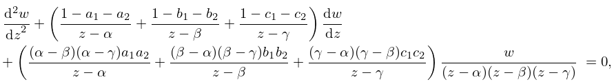
29: 15.11 Riemann’s Differential Equation

… ►The most general form is given by ►

15.11.1 $$\frac{d^{2}w}{{dz}^2}+\left(\frac{1-a_1-a_2}{z-\alpha }+\frac{1-b_1-b_2}{z-\beta }+\frac{1-c_1-c_2}{z-\gamma }\right)\frac{dw}{dz}+\left(\frac{(\alpha -\beta )(\alpha -\gamma )a_1{a}_2}{z-\alpha }+\frac{(\beta -\alpha )(\beta -\gamma )b_1{b}_2}{z-\beta }+\frac{(\gamma -\alpha )(\gamma -\beta )c_1{c}_2}{z-\gamma }\right)\frac{w}{(z-\alpha )(z-\beta )(z-\gamma )}=0,$$

ⓘ

Symbols:

$\frac{df}{dx}$: derivative of $f$ with respect to $x$ , $z$: complex variable, $a$: real or complex parameter, $b$: real or complex parameter, $c$: real or complex parameter, $\alpha$: point, $\beta$: point, $\gamma$: point and $w$: solution

Referenced by:

§15.11(i), §15.11(i), §15.17(v)

Permalink:

http://dlmf.nist.gov/15.11.E1

Encodings:

pMML, png, TeX

See also:

Annotations for §15.11(i), §15.11 and Ch.15

… ►Here $\{a_1,a_2\}$, $\{b_1,b_2\}$, $\{c_1,c_2\}$ are the exponent pairs at the points $\alpha$, $\beta$, $\gamma$, respectively. …Also, if any of $\alpha$, $\beta$, $\gamma$, is at infinity, then we take the corresponding limit in (15.11.1). … ►These constants can be chosen to map any two sets of three distinct points $\{\alpha ,\beta ,\gamma \}$ and $\{\tilde{\alpha },\tilde{\beta },\tilde{\gamma }\}$ onto each other. …

30: Sidebar 5.SB1: Gamma & Digamma Phase Plots

… ►The color encoded phases of $\mathrm{\Gamma }\left(z\right)$ (above) and $\psi \left(z\right)$ (below), are constrasted in the negative half of the complex plane. ►In the upper half of the image, the poles of $\mathrm{\Gamma }\left(z\right)$ are clearly visible at negative integer values of $z$: the phase changes by $2\pi$ around each pole, showing a full revolution of the color wheel. … ►In the lower half of the image, the poles of $\psi \left(z\right)$ (corresponding to the poles of $\mathrm{\Gamma }\left(z\right)$) and the zeros between them are clear. …