C. K. Chui (1988)Multivariate Splines.
CBMS-NSF Regional Conference Series in Applied Mathematics, Vol. 54, Society for Industrial and Applied Mathematics (SIAM), Philadelphia, PA.
►Splines are defined piecewise and usually by low-degree polynomials.
…
►For splines based on Bernoulli and Euler polynomials, see §24.17(ii).
…
►A complete spline results by composing several Bézier curves.
…See Knuth (1986, pp. 116-136).
R. Metzler, J. Klafter, and J. Jortner (1999)Hierarchies and logarithmic oscillations in the temporal relaxation patterns of proteins and other complex systems.
Proc. Nat. Acad. Sci. U .S. A.96 (20), pp. 11085–11089.
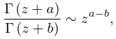
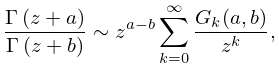
►As , with ,
…
►The asymptotic behavior of and as in descending powers of is derived in Meixner (1944).
…The asymptotic behavior of and as is given in Erdélyi et al. (1955, p. 151).
The behavior of for complex and large is investigated in Hunter and Guerrieri (1982).
…
…
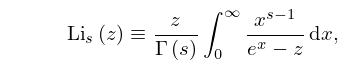
►The notation was introduced in Lewin (1981) for a function discussed in Euler (1768) and called the dilogarithm in Hill (1828):
…
►►►Figure 25.12.1: Dilogarithm function ,
Magnify►►
►Figure 25.12.2: Absolute value of the dilogarithm function , , .
…
Magnify3DHelp
…
►
►Bernoulli polynomials appear in statistical physics (Ordóñez and Driebe (1996)), in discussions of Casimir forces (Li et al. (1991)), and in a study of quark-gluon plasma (Meisinger et al. (2002)).
►Euler polynomials also appear in statistical physics as well as in semi-classical approximations to quantum probability distributions (Ballentine and McRae (1998)).
Cody et al. (1971) gives rational approximations for
in the form of quotients of polynomials or quotients of
Chebyshev series. The ranges covered are ,
, , . Precision is
varied, with a maximum of 20S.
Antia (1993) gives minimax rational approximations for
, where is the Fermi–Dirac integral
(25.12.14), for the intervals and
, with
. For each there
are three sets of approximations, with relative maximum errors
.
 ►
►
 ►
►
