Descartes’ rule of signs (for polynomials)

SearchAdvancedHelp

(0.002 seconds)

31—40 of 340 matching pages

31: Software Index

… ► ►►►►►

	Open Source													With Book						Commercial
…
18 Orthogonal Polynomials
…
24 Bernoulli and Euler Polynomials
24.21(ii) $B_n$, $B_n\left(x\right)$, $E_n$, $E_n\left(x\right)$	✓	✓						✓		✓		a	✓	✓			✓		✓		✓	✓	✓		Derive, MuPAD
…

… ►Please see our Software Indexing Policy for rules that govern the indexing of software in the DLMF. …

32: 24.18 Physical Applications

§24.18 Physical Applications

►Bernoulli polynomials appear in statistical physics (Ordóñez and Driebe (1996)), in discussions of Casimir forces (Li et al. (1991)), and in a study of quark-gluon plasma (Meisinger et al. (2002)). ►Euler polynomials also appear in statistical physics as well as in semi-classical approximations to quantum probability distributions (Ballentine and McRae (1998)).

33: 1.16 Distributions

… ►For a multi-index $𝜶=({\alpha }_1,{\alpha }_2,\mathrm{\dots },{\alpha }_n)$, define …Here $𝜶$ ranges over a finite set of multi-indices, $P(𝐱)$ is a multivariate polynomial, and $P(𝐃)$ is a partial differential operator. … ►

1.16.44 $$\mathrm{sign}\left(x\right)=2H\left(x\right)-1,$$ $x\ne 0$,

ⓘ

Symbols:

$H\left(x\right)$: Heaviside function and $\mathrm{sign}x$: sign of

Permalink:

http://dlmf.nist.gov/1.16.E44

Encodings:

pMML, png, TeX

See also:

Annotations for §1.16(viii), §1.16 and Ch.1

… ►and from (1.16.36) with $u=\mathrm{sign}$, $P(𝐃)=𝐷$, and $P_{-}(x)=-\mathrm{i}x$, we have also ►

1.16.47 $$ℱ\left({\mathrm{sign}}^{\prime }\right)=\frac{x}{\mathrm{i}}ℱ\left(\mathrm{sign}\right).$$

ⓘ

Symbols:

$ℱ\left(u\right)$: Fourier transform of a tempered distribution, $\mathrm{i}$: imaginary unit and $\mathrm{sign}x$: sign of

Referenced by:

§1.16(viii)

Permalink:

http://dlmf.nist.gov/1.16.E47

Encodings:

pMML, png, TeX

See also:

Annotations for §1.16(viii), §1.16 and Ch.1

…

34: 34.7 Basic Properties: $\mathit{9}j$ Symbol

… ►This equation is the sum rule. It constitutes an addition theorem for the $\mathit{9}j$ symbol. …

35: 5.11 Asymptotic Expansions

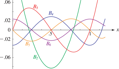
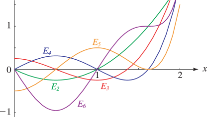
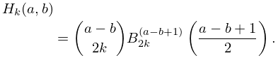
… ►where $h(\in ℂ)$ is fixed, and $B_k\left(h\right)$ is the Bernoulli polynomial defined in §24.2(i). … ►If the sums in the expansions (5.11.1) and (5.11.2) are terminated at $k=n-1$ ($k\ge 0$) and $z$ is real and positive, then the remainder terms are bounded in magnitude by the first neglected terms and have the same sign. … ►In terms of generalized Bernoulli polynomials $B_n^{(\mathrm{\ell })}\left(x\right)$ (§24.16(i)), we have for $k=0,1,\mathrm{\dots }$, ►

5.11.17 $$G_k(a,b)=\left(\genfrac{}{}{0.0pt}{}{a-b}{k}\right)B_k^{(a-b+1)}\left(a\right),$$

ⓘ

Defines:

$G_k(a,b)$: coefficients (locally)

Symbols:

$\left(\genfrac{}{}{0.0pt}{}{m}{n}\right)$: binomial coefficient, $B_n^{(\mathrm{\ell })}\left(x\right)$: generalized Bernoulli polynomials, $k$: nonnegative integer, $a$: real or complex variable and $b$: real or complex variable

Permalink:

http://dlmf.nist.gov/5.11.E17

Encodings:

pMML, png, TeX

See also:

Annotations for §5.11(iii), §5.11 and Ch.5

►

5.11.18 $$H_k(a,b)=\left(\genfrac{}{}{0.0pt}{}{a-b}{2k}\right)B_{2k}^{(a-b+1)}\left(\frac{a-b+1}{2}\right).$$

ⓘ

Defines:

$H_k(a,b)$: coefficients (locally)

Symbols:

$\left(\genfrac{}{}{0.0pt}{}{m}{n}\right)$: binomial coefficient, $B_n^{(\mathrm{\ell })}\left(x\right)$: generalized Bernoulli polynomials, $k$: nonnegative integer, $a$: real or complex variable and $b$: real or complex variable

Referenced by:

§5.11(iii)

Permalink:

http://dlmf.nist.gov/5.11.E18

Encodings:

pMML, png, TeX

See also:

Annotations for §5.11(iii), §5.11 and Ch.5

…

36: 15.9 Relations to Other Functions

… ►

§15.9(i) Orthogonal Polynomials

… ►

Jacobi

… ►

Meixner

… ►where the sign in the exponential is $\pm$ according as $\mathrm{\Im }z\gtrless 0$. …where the sign in the exponential is $\pm$ according as $\mathrm{\Im }z\gtrless 0$. …

37: Sidebar 5.SB1: Gamma & Digamma Phase Plots

… ►Phase changes around the zeros are of opposite sign to those around the poles. The fluid flow analogy in this case involves a line of vortices of alternating sign of circulation, resulting in a near cancellation of flow far from the real axis.

38: 28.31 Equations of Whittaker–Hill and Ince

… ►

§28.31(ii) Equation of Ince; Ince Polynomials

… ► … ►The normalization is given by …ambiguities in sign being resolved by requiring $C_p^m(x,\xi )$ and $S_p^m{}_{}{}^{\prime }(x,\xi )$ to be continuous functions of $x$ and positive when $x=0$. … ►For change of sign of $\xi$, …

39: 19.14 Reduction of General Elliptic Integrals

… ►

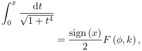
19.14.3 $${\int }_0^x\frac{dt}{\sqrt{1+t^4}}=\frac{\mathrm{sign}\left(x\right)}{2}F(\varphi ,k),$$ $\cos \varphi ={\displaystyle \frac{1-x^2}{1+x^2}}$, $k^2={\displaystyle \frac{1}{2}}$.

ⓘ

Symbols:

$\cos z$: cosine function, $dx$: differential of $x$ , $F(\varphi ,k)$: Legendre’s incomplete elliptic integral of the first kind, $\int$: integral, $\mathrm{sign}x$: sign of, $\varphi$: real or complex argument and $k$: real or complex modulus

Referenced by:

§19.14(i)

Permalink:

http://dlmf.nist.gov/19.14.E3

Encodings:

pMML, png, TeX

See also:

Annotations for §19.14(i), §19.14 and Ch.19

… ►In (19.14.4) , each quadratic polynomial is positive on the interval $(y,x)$, and $\alpha ,\beta ,\gamma$ is a permutation of $0,a_1{b}_2,a_2{b}_1$ (not all 0 by assumption) such that $\alpha \le \beta \le \gamma$. … ►The choice among 21 transformations for final reduction to Legendre’s normal form depends on inequalities involving the limits of integration and the zeros of the cubic or quartic polynomial. …

40: 24.3 Graphs

… ►

►►

Figure 24.3.1: Bernoulli polynomials $B_n\left(x\right)$, $n=2,3,\mathrm{\dots },6$. Magnify

►

►►

Figure 24.3.2: Euler polynomials $E_n\left(x\right)$, $n=2,3,\mathrm{\dots },6$. Magnify