Džrbasjan sum

SearchAdvancedHelp

The term"rbasjan" was not found.Possible alternative term: "džrbasjan".

(0.002 seconds)

1—10 of 411 matching pages

1: 26.10 Integer Partitions: Other Restrictions

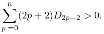
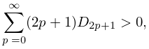
… ► $p(𝒟,n)$ denotes the number of partitions of $n$ into distinct parts. $p_m(𝒟,n)$ denotes the number of partitions of $n$ into at most $m$ distinct parts. $p(𝒟k,n)$ denotes the number of partitions of $n$ into parts with difference at least $k$. …If more than one restriction applies, then the restrictions are separated by commas, for example, $p(𝒟2,\in T,n)$. … ►Note that $p({𝒟}^{\prime }3,n)\le p(𝒟3,n)$, with strict inequality for $n\ge 9$. …

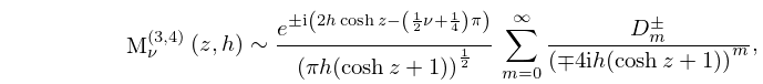
2: 28.25 Asymptotic Expansions for Large $\mathrm{\Re }z$

… ►

28.25.1 $${\mathrm{M}}_{\nu }^{(3,4)}(z,h)\sim \frac{{\mathrm{e}}^{\pm \mathrm{i}\left(2h\cosh z-\left(\frac{1}{2}\nu +\frac{1}{4}\right)\pi \right)}}{{\left(\pi h(\cosh z+1)\right)}^{\frac{1}{2}}}\sum _{m=0}^{\mathrm{\infty }}\frac{D_m^{\pm }}{{\left(\mp 4\mathrm{i}h(\cosh z+1)\right)}^m},$$

ⓘ

Symbols:

$\sim$: Poincaré asymptotic expansion, $\pi$: the ratio of the circumference of a circle to its diameter, $\mathrm{e}$: base of natural logarithm, $\cosh z$: hyperbolic cosine function, $\mathrm{i}$: imaginary unit, ${\mathrm{M}}_{\nu }^{(j)}(z,h)$: modified Mathieu function, $m$: integer, $h$: parameter, $z$: complex variable, $\nu$: complex parameter and $D_m^{\pm }$: coefficients

A&S Ref:

20.9.1 (for 3 and for integer $\nu$) 20.9.3 (for 4 and for integer $\nu$)

Referenced by:

§28.25

Permalink:

http://dlmf.nist.gov/28.25.E1

Encodings:

pMML, png, TeX

See also:

Annotations for §28.25 and Ch.28

… ►

$D_{-1}^{\pm }=0,$

►

$D_0^{\pm }=1,$

… ►

28.25.3 $$(m+1)D_{m+1}^{\pm }+\left({(m+\frac{1}{2})}^2\pm (m+\frac{1}{4})8\mathrm{i}h+2h^2-a\right)D_m^{\pm }\pm (m-\frac{1}{2})\left(8\mathrm{i}hm\right)D_{m-1}^{\pm }=0,$$ $m\ge 0$.

ⓘ

Symbols:

$\mathrm{i}$: imaginary unit, $m$: integer, $h$: parameter, $a$: parameter and $D_m^{\pm }$: coefficients

A&S Ref:

20.9.2 (for $+$) 20.9.4 (for $-$)

Permalink:

http://dlmf.nist.gov/28.25.E3

Encodings:

pMML, png, TeX

See also:

Annotations for §28.25 and Ch.28

…

3: 1.10 Functions of a Complex Variable

… ►Let $D$ be a bounded domain with boundary $\partial D$ and let $\overline{D}=D\cup \partial D$. … ►If $u(z)$ is harmonic in $D$, $z_0\in D$, and $u(z)\le u(z_0)$ for all $z\in D$, then $u(z)$ is constant in $D$. Moreover, if $D$ is bounded and $u(z)$ is continuous on $\overline{D}$ and harmonic in $D$, then $u(z)$ is maximum at some point on $\partial D$. … ►Let $F(z)$ be a multivalued function and $D$ be a domain. … ►Suppose $D$ is a domain, and …

4: 19.21 Connection Formulas

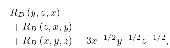
… ►The complete case of $R_J$ can be expressed in terms of $R_F$ and $R_D$: … ► $R_D(x,y,z)$ is symmetric only in $x$ and $y$, but either (nonzero) $x$ or (nonzero) $y$ can be moved to the third position by using … ►

19.21.8 $$R_D(y,z,x)+R_D(z,x,y)+R_D(x,y,z)=3x^{-1/2}{y}^{-1/2}{z}^{-1/2},$$

ⓘ

Symbols:

$R_D(x,y,z)$: elliptic integral symmetric in only two variables

Referenced by:

§19.21(ii), §19.33(iii), Erratum (V1.1.3) for Chapter 19

Permalink:

http://dlmf.nist.gov/19.21.E8

Encodings:

pMML, png, TeX

Correction (effective with 1.1.3):

The factors inside the square root on the right-hand side were written as products to ensure the correct multivalued behavior.

Suggested 2021-06-07 by Luc Maisonobe

See also:

Annotations for §19.21(ii), §19.21 and Ch.19

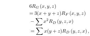
… ►Because $R_G$ is completely symmetric, $x,y,z$ can be permuted on the right-hand side of (19.21.10) so that $(x-z)(y-z)\le 0$ if the variables are real, thereby avoiding cancellations when $R_G$ is calculated from $R_F$ and $R_D$ (see §19.36(i)). ►

19.21.11 $$6R_G(x,y,z)=3(x+y+z)R_F(x,y,z)-\sum x^2{R}_D(y,z,x)=\sum x(y+z)R_D(y,z,x),$$

ⓘ

Symbols:

$R_D(x,y,z)$: elliptic integral symmetric in only two variables, $R_F(x,y,z)$: symmetric elliptic integral of first kind and $R_G(x,y,z)$: symmetric elliptic integral of second kind

Referenced by:

§19.21(i), §19.21(ii)

Permalink:

http://dlmf.nist.gov/19.21.E11

Encodings:

pMML, png, TeX

See also:

Annotations for §19.21(ii), §19.21 and Ch.19

…

5: 26.6 Other Lattice Path Numbers

… ►

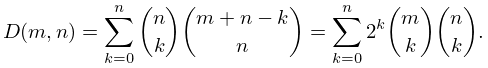
Delannoy Number $D(m,n)$

► $D(m,n)$ is the number of paths from $(0,0)$ to $(m,n)$ that are composed of directed line segments of the form $(1,0)$, $(0,1)$, or $(1,1)$. ►

26.6.1 $$D(m,n)=\sum _{k=0}^n\left(\genfrac{}{}{0.0pt}{}{n}{k}\right)\left(\genfrac{}{}{0.0pt}{}{m+n-k}{n}\right)=\sum _{k=0}^n{2}^k\left(\genfrac{}{}{0.0pt}{}{m}{k}\right)\left(\genfrac{}{}{0.0pt}{}{n}{k}\right).$$

ⓘ

Defines:

$D(m,n)$: Delannoy number (locally)

Symbols:

$\left(\genfrac{}{}{0.0pt}{}{m}{n}\right)$: binomial coefficient, $k$: nonnegative integer, $m$: nonnegative integer and $n$: nonnegative integer

Permalink:

http://dlmf.nist.gov/26.6.E1

Encodings:

pMML, png, TeX

See also:

Annotations for §26.6(i), §26.6(i), §26.6 and Ch.26

… ►

26.6.5 $$\sum _{m,n=0}^{\mathrm{\infty }}D(m,n)x^m{y}^n=\frac{1}{1-x-y-xy},$$

ⓘ

Symbols:

$m$: nonnegative integer, $n$: nonnegative integer, $D(m,n)$: Delannoy number, $x$: small and $y$: small

Permalink:

http://dlmf.nist.gov/26.6.E5

Encodings:

pMML, png, TeX

See also:

Annotations for §26.6(ii), §26.6 and Ch.26

►

26.6.6 $$\sum _{n=0}^{\mathrm{\infty }}D(n,n)x^n=\frac{1}{\sqrt{1-6x+x^2}},$$

ⓘ

Symbols:

$n$: nonnegative integer, $D(m,n)$: Delannoy number and $x$: small

Permalink:

http://dlmf.nist.gov/26.6.E6

Encodings:

pMML, png, TeX

See also:

Annotations for §26.6(ii), §26.6 and Ch.26

…

6: 1.16 Distributions

… ►We denote it by $𝒟(I)$. … ►for all $\varphi \in 𝒟(I)$. … ►If $f$ is a locally integrable function then its distributional derivative is $𝐷f={\mathrm{\Lambda }}_f^{\prime }$. … ►The distributional derivative ${𝐷}^{k}f$ of $f$ is defined by …

7: 29.15 Fourier Series and Chebyshev Series

… ►

29.15.34 $${[D_1,D_3,\mathrm{\dots },D_{2n+1}]}^{\mathrm{T}},$$

ⓘ

Symbols:

$n$: nonnegative integer and $D_{2p}$: coefficents

Permalink:

http://dlmf.nist.gov/29.15.E34

Encodings:

pMML, png, TeX

See also:

Annotations for §29.15(i), §29.15(i), §29.15 and Ch.29

►

29.15.35 $$\left(1-\frac{1}{2}{k}^2\right)\sum _{p=0}^n{D}_{2p+1}^2+\frac{1}{2}{k}^2\left(\frac{1}{2}{D}_1^2-\sum _{p=0}^{n-1}{D}_{2p+1}{D}_{2p+3}\right)=1,$$

ⓘ

Symbols:

$n$: nonnegative integer, $p$: nonnegative integer, $k$: real parameter and $D_{2p}$: coefficents

Permalink:

http://dlmf.nist.gov/29.15.E35

Encodings:

pMML, png, TeX

See also:

Annotations for §29.15(i), §29.15(i), §29.15 and Ch.29

►

29.15.36 $$\sum _{p=0}^n(2p+1)D_{2p+1}>0.$$

ⓘ

Symbols:

$n$: nonnegative integer, $p$: nonnegative integer and $D_{2p}$: coefficents

Permalink:

http://dlmf.nist.gov/29.15.E36

Encodings:

pMML, png, TeX

See also:

Annotations for §29.15(i), §29.15(i), §29.15 and Ch.29

… ►

29.15.40 $$\left(1-\frac{1}{2}{k}^2\right)\sum _{p=0}^n{D}_{2p+2}^2-\frac{1}{2}{k}^2\sum _{p=1}^n{D}_{2p}{D}_{2p+2}=1,$$

ⓘ

Symbols:

$n$: nonnegative integer, $p$: nonnegative integer, $k$: real parameter and $D_{2p}$: coefficents

Permalink:

http://dlmf.nist.gov/29.15.E40

Encodings:

pMML, png, TeX

See also:

Annotations for §29.15(i), §29.15(i), §29.15 and Ch.29

►

29.15.41 $$\sum _{p=0}^n(2p+2)D_{2p+2}>0.$$

ⓘ

Symbols:

$n$: nonnegative integer, $p$: nonnegative integer and $D_{2p}$: coefficents

Permalink:

http://dlmf.nist.gov/29.15.E41

Encodings:

pMML, png, TeX

See also:

Annotations for §29.15(i), §29.15(i), §29.15 and Ch.29

…

8: 29.6 Fourier Series

… ►

29.6.42 $$\left(1-\frac{1}{2}{k}^2\right)\sum _{p=0}^{\mathrm{\infty }}{D}_{2p+1}^2+\frac{1}{2}{k}^2\left(\frac{1}{2}{D}_1^2-\sum _{p=0}^{\mathrm{\infty }}{D}_{2p+1}{D}_{2p+3}\right)=1,$$

ⓘ

Symbols:

$p$: nonnegative integer, $k$: real parameter and $D_{2p+1}$: coefficents

Permalink:

http://dlmf.nist.gov/29.6.E42

Encodings:

pMML, png, TeX

See also:

Annotations for §29.6(iii), §29.6 and Ch.29

►

29.6.43 $$\sum _{p=0}^{\mathrm{\infty }}(2p+1)D_{2p+1}>0,$$

ⓘ

Symbols:

$p$: nonnegative integer and $D_{2p+1}$: coefficents

Permalink:

http://dlmf.nist.gov/29.6.E43

Encodings:

pMML, png, TeX

See also:

Annotations for §29.6(iii), §29.6 and Ch.29

… ►

29.6.53 $${\mathrm{𝐸𝑠}}_{\nu }^{2m+2}(z,k^2)=\mathrm{dn}(z,k)\sum _{p=1}^{\mathrm{\infty }}{D}_{2p}\sin \left(2p\varphi \right),$$

ⓘ

Symbols:

$\mathrm{dn}(z,k)$: Jacobian elliptic function, ${\mathrm{𝐸𝑠}}_{\nu }^m(z,k^2)$: Lamé function, $\sin z$: sine function, $m$: nonnegative integer, $p$: nonnegative integer, $z$: complex variable, $k$: real parameter, $\nu$: real parameter, $\varphi$: change of variable and $D_{2p}$: coefficents

Referenced by:

§29.15(i)

Permalink:

http://dlmf.nist.gov/29.6.E53

Encodings:

pMML, png, TeX

See also:

Annotations for §29.6(iv), §29.6 and Ch.29

… ►

29.6.57 $$\left(1-\frac{1}{2}{k}^2\right)\sum _{p=1}^{\mathrm{\infty }}{D}_{2p}^2-\frac{1}{2}{k}^2\sum _{p=1}^{\mathrm{\infty }}{D}_{2p}{D}_{2p+2}=1,$$

ⓘ

Symbols:

$p$: nonnegative integer, $k$: real parameter and $D_{2p}$: coefficents

Permalink:

http://dlmf.nist.gov/29.6.E57

Encodings:

pMML, png, TeX

See also:

Annotations for §29.6(iv), §29.6 and Ch.29

►

29.6.58 $$\sum _{p=0}^{\mathrm{\infty }}(2p+2)D_{2p+2}>0,$$

ⓘ

Symbols:

$p$: nonnegative integer and $D_{2p}$: coefficents

Permalink:

http://dlmf.nist.gov/29.6.E58

Encodings:

pMML, png, TeX

See also:

Annotations for §29.6(iv), §29.6 and Ch.29

…

9: 1.11 Zeros of Polynomials

… ►

$D=b^2-4ac.$

►The sum and product of the roots are respectively $-b/a$ and $c/a$. … ►Let ►

$D_1=a_1,$

… ►Then $f(z)$, with $a_n\ne 0$, is stable iff $a_0\ne 0$; $D_{2k}>0$, $k=1,\mathrm{\dots },\lfloor \frac{1}{2}n\rfloor$; $\mathrm{sign}{D}_{2k+1}=\mathrm{sign}{a}_0$, $k=0,1,\mathrm{\dots },\lfloor \frac{1}{2}n-\frac{1}{2}\rfloor$.

10: 10.20 Uniform Asymptotic Expansions for Large Order

… ►In the following formulas for the coefficients $A_k(\zeta )$, $B_k(\zeta )$, $C_k(\zeta )$, and $D_k(\zeta )$, $u_k$, $v_k$ are the constants defined in §9.7(i), and $U_k(p)$, $V_k(p)$ are the polynomials in $p$ of degree $3k$ defined in §10.41(ii). … ►Note: Another way of arranging the above formulas for the coefficients $A_k(\zeta ),B_k(\zeta ),C_k(\zeta )$, and $D_k(\zeta )$ would be by analogy with (12.10.42) and (12.10.46). … ►Each of the coefficients $A_k(\zeta )$, $B_k(\zeta )$, $C_k(\zeta )$, and $D_k(\zeta )$, $k=0,1,2,\mathrm{\dots }$, is real and infinitely differentiable on the interval . … ►For numerical tables of $\zeta =\zeta (z)$, ${(4\zeta /(1-z^2))}^{\frac{1}{4}}$ and $A_k(\zeta )$, $B_k(\zeta )$, $C_k(\zeta )$, and $D_k(\zeta )$ see Olver (1962, pp. 28–42). … ►The equations of the curved boundaries $D_1{E}_1$ and $D_2{E}_2$ in the $\zeta$-plane are given parametrically by …