Cayley identity for Schwarzian derivatives

(0.003 seconds)

11—20 of 366 matching pages

11: 9.18 Tables

… ►

•

Yakovleva (1969) tabulates Fock’s functions $U(x)\equiv\sqrt{\pi}\operatorname{Bi}\left(x\right)$ , $U^{\prime}(x)=\sqrt{\pi}\operatorname{Bi}'\left(x\right)$ , $V(x)\equiv\sqrt{\pi}\operatorname{Ai}\left(x\right)$ , $V^{\prime}(x)=\sqrt{\pi}\operatorname{Ai}'\left(x\right)$ for $x=-9(.001)9$ . Precision is 7S.

… ►

•

Miller (1946) tabulates $a_{k}$ , $\operatorname{Ai}'\left(a_{k}\right)$ , $a^{\prime}_{k}$ , $\operatorname{Ai}\left(a^{\prime}_{k}\right)$ , $k=1(1)50$ ; $b_{k}$ , $\operatorname{Bi}'\left(b_{k}\right)$ , $b^{\prime}_{k}$ , $\operatorname{Bi}\left(b^{\prime}_{k}\right)$ , $k=1(1)20$ . Precision is 8D. Entries for $k=1(1)20$ are reproduced in Abramowitz and Stegun (1964, Chapter 10).

►

•

Sherry (1959) tabulates $a_{k}$ , $\operatorname{Ai}'\left(a_{k}\right)$ , $a^{\prime}_{k}$ , $\operatorname{Ai}\left(a^{\prime}_{k}\right)$ , $k=1(1)50$ ; 20S.

… ►

•

National Bureau of Standards (1958) tabulates $A_{0}(x)\equiv\pi\operatorname{Hi}\left(-x\right)$ and $-A_{0}^{\prime}(x)\equiv\pi\operatorname{Hi}'\left(-x\right)$ for $x=0(.01)1(.02)5(.05)11$ and $1/x=0.01(.01)0.1$ ; $\int_{0}^{x}A_{0}(t)\,\mathrm{d}t$ for $x=0.5,1(1)11$ . Precision is 8D.

►

•

Nosova and Tumarkin (1965) tabulates $e_{0}(x)\equiv\pi\operatorname{Hi}\left(-x\right)$ , $e^{\prime}_{0}(x)=-\pi\operatorname{Hi}'\left(-x\right)$ , $\widetilde{e}_{0}(-x)\equiv-\pi\operatorname{Gi}\left(x\right)$ , $\widetilde{e}^{\mspace{2.0mu}\prime}_{0}(-x)=\pi\operatorname{Gi}'\left(x\right)$ for $x=-1(.01)10$ ; 7D. Also included are the real and imaginary parts of $e_{0}(z)$ and $ie^{\prime}_{0}(z)$ , where $z=iy$ and $y=0(.01)9$ ; 6-7D.

…

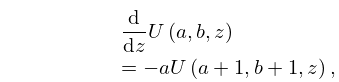
12: 13.3 Recurrence Relations and Derivatives

§13.3 Recurrence Relations and Derivatives

… ►

§13.3(ii) Differentiation Formulas

… ►

13.3.22

\frac{\mathrm{d}}{\mathrm{d}z}U\left(a,b,z\right)=-aU\left(a+1,b+1,z\right),

ⓘ

Symbols:: $U\left(\NVar{a},\NVar{b},\NVar{z}\right)$ : Kummer confluent hypergeometric function, $\frac{\mathrm{d}\NVar{f}}{\mathrm{d}\NVar{x}}$ : derivative of $f$ with respect to $x$ and $z$ : complex variable
A&S Ref:: 13.4.21
Permalink:: http://dlmf.nist.gov/13.3.E22
Encodings:: pMML, png, TeX
See also:: Annotations for §13.3(ii), §13.3 and Ch.13

… ►Other versions of several of the identities in this subsection can be constructed with the aid of the operator identity ►

13.3.29

\left(z\frac{\mathrm{d}}{\mathrm{d}z}z\right)^{n}=z^{n}\frac{{\mathrm{d}}^{n}}% {{\mathrm{d}z}^{n}}z^{n},

n=1,2,3,\dots

ⓘ

Symbols:: $\frac{\mathrm{d}\NVar{f}}{\mathrm{d}\NVar{x}}$ : derivative of $f$ with respect to $x$ , $n$ : nonnegative integer and $z$ : complex variable
Referenced by:: §13.15(ii), §13.3(ii)
Permalink:: http://dlmf.nist.gov/13.3.E29
Encodings:: pMML, png, TeX
See also:: Annotations for §13.3(ii), §13.3 and Ch.13

13: 27.14 Unrestricted Partitions

… ►

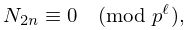
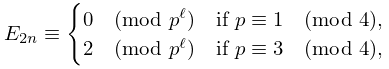
§27.14(v) Divisibility Properties

►Ramanujan (1921) gives identities that imply divisibility properties of the partition function. For example, the Ramanujan identity …implies

p\left(5n+4\right)\equiv 0\pmod{5}

. …For example,

p\left(1575\;25693n+1\;11247\right)\equiv 0\pmod{13}

. …

14: 24.10 Arithmetic Properties

… ►where

m\equiv n\not\equiv 0\pmod{p-1}

. …valid when

m\equiv n\pmod{(p-1)p^{\ell}}

and

n\not\equiv 0\pmod{p-1}

, where

\ell(\geq 0)

is a fixed integer. … ►

24.10.8

N_{2n}\equiv 0\pmod{p^{\ell}},

ⓘ

Symbols:: $\equiv$ : modular equivalence, $\ell$ : integer, $n$ : integer and $p$ : prime
Referenced by:: §24.10(iv)
Permalink:: http://dlmf.nist.gov/24.10.E8
Encodings:: pMML, png, TeX
See also:: Annotations for §24.10(iv), §24.10 and Ch.24

►valid for fixed integers

\ell(\geq 1)

, and for all

n(\geq 1)

such that

2n\not\equiv 0

\pmod{p-1}

and

p^{\ell}\mathbin{|}2n

. ►

24.10.9

E_{2n}\equiv\begin{cases}0\pmod{p^{\ell}}&\text{if }p\equiv 1\pmod{4},\\ 2\pmod{p^{\ell}}&\text{if }p\equiv 3\pmod{4},\end{cases}

ⓘ

Symbols:: $E_{\NVar{n}}$ : Euler numbers, $\equiv$ : modular equivalence, $\ell$ : integer, $n$ : integer and $p$ : prime
Referenced by:: §24.10(iv)
Permalink:: http://dlmf.nist.gov/24.10.E9
Encodings:: pMML, png, TeX
See also:: Annotations for §24.10(iv), §24.10 and Ch.24

…

15: 20.4 Values at $z$ = 0

§20.4 Values at $z$ = 0

►

§20.4(i) Functions and First Derivatives

… ►

Jacobi’s Identity

… ►

§20.4(ii) Higher Derivatives

…

16: 19.11 Addition Theorems

…

17: 20.7 Identities

§20.7 Identities

… ►Also, in further development along the lines of the notations of Neville (§20.1) and of Glaisher (§22.2), the identities (20.7.6)–(20.7.9) have been recast in a more symmetric manner with respect to suffices

2,3,4

. … ►

§20.7(v) Watson’s Identities

… ►

§20.7(vii) Derivatives of Ratios of Theta Functions

… ►This reference also gives the eleven additional identities for the permutations of the four theta functions. …

18: 16.19 Identities

§16.19 Identities

… ►where again

\vartheta=z\ifrac{\mathrm{d}}{\mathrm{d}z}

. …This reference and Mathai (1993, §§2.2 and 2.4) also supply additional identities.

19: Errata

… ►

Equation (25.15.6)

25.15.6

G(\chi)\equiv\sum_{r=1}^{k-1}\chi(r){\mathrm{e}}^{2\pi ir/k}.

The upper-index of the finite sum which originally was $k$ , was replaced with $k-1$ since $\chi(k)=0$ .

Reported by Gergő Nemes on 2021-08-23

… ►

Section 1.13

In Equation (1.13.4), the determinant form of the two-argument Wronskian

1.13.4

\mathscr{W}\left\{w_{1}(z),w_{2}(z)\right\}=\det\begin{bmatrix}w_{1}(z)&w_{2}(% z)\\ w_{1}^{\prime}(z)&w_{2}^{\prime}(z)\end{bmatrix}=w_{1}(z)w_{2}^{\prime}(z)-w_{% 2}(z)w_{1}^{\prime}(z)

was added as an equality. In ¶Wronskian (in §1.13(i)), immediately below Equation (1.13.4), a sentence was added indicating that in general the $n$ -argument Wronskian is given by $\mathscr{W}\left\{w_{1}(z),\ldots,w_{n}(z)\right\}=\det\left[w_{k}^{(j-1)}(z)\right]$ , where $1\leq j,k\leq n$ . Immediately below Equation (1.13.4), a sentence was added giving the definition of the $n$ -argument Wronskian. It is explained just above (1.13.5) that this equation is often referred to as Abel’s identity. Immediately below Equation (1.13.5), a sentence was added explaining how it generalizes for $n$ th-order differential equations. A reference to Ince (1926, §5.2) was added.

… ►

Subsection 19.11(i)

A sentence and unnumbered equation

R_{C}\left(\gamma-\delta,\gamma\right)=\frac{-1}{\sqrt{\delta}}\operatorname{% arctan}\left(\frac{\sqrt{\delta}\sin\theta\sin\phi\sin\psi}{\alpha^{2}-1-% \alpha^{2}\cos\theta\cos\phi\cos\psi}\right),

were added which indicate that care must be taken with the multivalued functions in (19.11.5). See (Cayley, 1961, pp. 103-106).

Suggested by Albert Groenenboom.

… ►

Notation

The overloaded operator $\equiv$ is now more clearly separated (and linked) to two distinct cases: equivalence by definition (in §§1.4(ii), 1.4(v), 2.7(i), 2.10(iv), 3.1(i), 3.1(iv), 4.18, 9.18(ii), 9.18(vi), 9.18(vi), 18.2(iv), 20.2(iii), 20.7(vi), 23.20(ii), 25.10(i), 26.15, 31.17(i)); and modular equivalence (in §§24.10(i), 24.10(ii), 24.10(iii), 24.10(iv), 24.15(iii), 24.19(ii), 26.14(i), 26.21, 27.2(i), 27.8, 27.9, 27.11, 27.12, 27.14(v), 27.14(vi), 27.15, 27.16, 27.19).

… ►

Subsection 5.2(iii)

Three new identities for Pochhammer’s symbol (5.2.6)–(5.2.8) have been added at the end of this subsection.

Suggested by Tom Koornwinder.

…

20: 15.5 Derivatives and Contiguous Functions

§15.5 Derivatives and Contiguous Functions

►

§15.5(i) Differentiation Formulas