Catalan%20constant

SearchAdvancedHelp

(0.002 seconds)

11—20 of 498 matching pages

11: 30.9 Asymptotic Approximations and Expansions

… ►

§30.9(i) Prolate Spheroidal Wave Functions

►As ${\gamma }^2\to +\mathrm{\infty }$, with $q=2(n-m)+1$, … ►The asymptotic behavior of ${\lambda }_n^m\left({\gamma }^2\right)$ and $a_{n,k}^m({\gamma }^2)$ as $n\to \mathrm{\infty }$ in descending powers of $2n+1$ is derived in Meixner (1944). …The asymptotic behavior of ${\mathrm{𝖯𝗌}}_n^m(x,{\gamma }^2)$ and ${\mathrm{𝖰𝗌}}_n^m(x,{\gamma }^2)$ as $x\to \pm 1$ is given in Erdélyi et al. (1955, p. 151). The behavior of ${\lambda }_n^m\left({\gamma }^2\right)$ for complex ${\gamma }^2$ and large $|{\lambda }_n^m\left({\gamma }^2\right)|$ is investigated in Hunter and Guerrieri (1982). …

12: 8 Incomplete Gamma and Related
Functions

…

13: 28 Mathieu Functions and Hill’s Equation

…

14: 23 Weierstrass Elliptic and Modular
Functions

…

15: 36.5 Stokes Sets

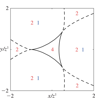
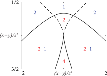
… ►where $j$ denotes a real critical point (36.4.1) or (36.4.2), and $\mu$ denotes a critical point with complex $t$ or $s,t$, connected with $j$ by a steepest-descent path (that is, a path where $\mathrm{\Re }\mathrm{\Phi }=\mathrm{constant}$) in complex $t$ or $(s,t)$ space. … ►

36.5.4 $$80x^5-40x^4-55x^3+5x^2+20x-1=0,$$

ⓘ

Symbols:

$x$: real parameter

Permalink:

http://dlmf.nist.gov/36.5.E4

Encodings:

pMML, png, TeX

See also:

Annotations for §36.5(ii), §36.5(ii), §36.5 and Ch.36

… ►

36.5.7 $$X=\frac{9}{20}+20u^4-\frac{Y^2}{20u^2}+6u^2\mathrm{sign}\left(z\right),$$

ⓘ

Symbols:

$\mathrm{sign}x$: sign of, $z$: real parameter, $X$: scaled coordinate and $Y$: scaled coordinate

Permalink:

http://dlmf.nist.gov/36.5.E7

Encodings:

pMML, png, TeX

See also:

Annotations for §36.5(ii), §36.5(ii), §36.5 and Ch.36

… ►

►►

Figure 36.5.5: Elliptic umbilic catastrophe with $z=\mathrm{constant}$. … Magnify

►

►►

Figure 36.5.6: Hyperbolic umbilic catastrophe with $z=\mathrm{constant}$. Magnify

…

16: 11.6 Asymptotic Expansions

… ►

11.6.1 $${𝐊}_{\nu }\left(z\right)\sim \frac{1}{\pi }\sum _{k=0}^{\mathrm{\infty }}\frac{\mathrm{\Gamma }\left(k+\frac{1}{2}\right){(\frac{1}{2}z)}^{\nu -2k-1}}{\mathrm{\Gamma }\left(\nu +\frac{1}{2}-k\right)},$$ $|\mathrm{ph}z|\le \pi -\delta$,

ⓘ

Symbols:

$\mathrm{\Gamma }\left(z\right)$: gamma function, ${𝐊}_{\nu }\left(z\right)$: Struve function, $\sim$: Poincaré asymptotic expansion, $\pi$: the ratio of the circumference of a circle to its diameter, $\mathrm{ph}$: phase, $z$: complex variable, $\nu$: real or complex order, $k$: nonnegative integer and $\delta$: arbitrary small positive constant

A&S Ref:

12.1.29

Referenced by:

§11.6(i), §11.6(i), §11.6(i), §11.6(i)

Permalink:

http://dlmf.nist.gov/11.6.E1

Encodings:

pMML, png, TeX

See also:

Annotations for §11.6(i), §11.6 and Ch.11

►where $\delta$ is an arbitrary small positive constant. … ►

11.6.2 $${𝐌}_{\nu }\left(z\right)\sim \frac{1}{\pi }\sum _{k=0}^{\mathrm{\infty }}{(-1)}^{k+1}\frac{\mathrm{\Gamma }\left(k+\frac{1}{2}\right){(\frac{1}{2}z)}^{\nu -2k-1}}{\mathrm{\Gamma }\left(\nu +\frac{1}{2}-k\right)},$$ $|\mathrm{ph}z|\le \frac{1}{2}\pi -\delta$.

ⓘ

Symbols:

$\mathrm{\Gamma }\left(z\right)$: gamma function, ${𝐌}_{\nu }\left(z\right)$: modified Struve function, $\sim$: Poincaré asymptotic expansion, $\pi$: the ratio of the circumference of a circle to its diameter, $\mathrm{ph}$: phase, $z$: complex variable, $\nu$: real or complex order, $k$: nonnegative integer and $\delta$: arbitrary small positive constant

A&S Ref:

12.2.6

Referenced by:

§11.6(i), §11.6(i), §11.6(i)

Permalink:

http://dlmf.nist.gov/11.6.E2

Encodings:

pMML, png, TeX

See also:

Annotations for §11.6(i), §11.6 and Ch.11

… ►where $\gamma$ is Euler’s constant (§5.2(ii)). … ►

$c_3(\lambda )=20{\lambda }^{-6}-4{\lambda }^{-4},$

…

17: 5.11 Asymptotic Expansions

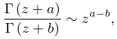
… ►The scaled gamma function ${\mathrm{\Gamma }}^{\ast }\left(z\right)$ is defined in (5.11.3) and its main property is ${\mathrm{\Gamma }}^{\ast }\left(z\right)\sim 1$ as $z\to \mathrm{\infty }$ in the sector $|\mathrm{ph}z|\le \pi -\delta$. Wrench (1968) gives exact values of $g_k$ up to $g_{20}$. … ►In this subsection $a$, $b$, and $c$ are real or complex constants. … ►

5.11.12 $$\frac{\mathrm{\Gamma }\left(z+a\right)}{\mathrm{\Gamma }\left(z+b\right)}\sim z^{a-b},$$

ⓘ

Symbols:

$\mathrm{\Gamma }\left(z\right)$: gamma function, $\sim$: asymptotic equality, $z$: complex variable, $a$: real or complex variable and $b$: real or complex variable

Referenced by:

§5.11(i)

Permalink:

http://dlmf.nist.gov/5.11.E12

Encodings:

pMML, png, TeX

See also:

Annotations for §5.11(iii), §5.11 and Ch.5

… ►

5.11.19 $$\frac{\mathrm{\Gamma }\left(z+a\right)\mathrm{\Gamma }\left(z+b\right)}{\mathrm{\Gamma }\left(z+c\right)}\sim \sum _{k=0}^{\mathrm{\infty }}{(-1)}^k\frac{{\left(c-a\right)}_k{\left(c-b\right)}_k}{k!}\mathrm{\Gamma }\left(a+b-c+z-k\right).$$

ⓘ

Symbols:

$\mathrm{\Gamma }\left(z\right)$: gamma function, ${\left(a\right)}_n$: Pochhammer’s symbol (or shifted factorial), $\sim$: Poincaré asymptotic expansion, $!$: factorial (as in $n!$), $k$: nonnegative integer, $z$: complex variable, $a$: real or complex variable and $b$: real or complex variable

Referenced by:

§5.11(i), §5.11(iii)

Permalink:

http://dlmf.nist.gov/5.11.E19

Encodings:

pMML, png, TeX

See also:

Annotations for §5.11(iii), §5.11 and Ch.5

…

18: 25.6 Integer Arguments

… ►

25.6.3 $$\zeta \left(-n\right)=-\frac{B_{n+1}}{n+1},$$ $n=1,2,3,\mathrm{\dots }$.

ⓘ

Symbols:

$B_n$: Bernoulli numbers, $\zeta \left(s\right)$: Riemann zeta function and $n$: nonnegative integer

Source:

Apostol (1976, (20), p. 266); with $n\ne 0$

A&S Ref:

23.2.15 (in slightly different form)

Permalink:

http://dlmf.nist.gov/25.6.E3

Encodings:

pMML, png, TeX

See also:

Annotations for §25.6(i), §25.6 and Ch.25

… ►

25.6.12 $${\zeta }^{\prime \prime }\left(0\right)=-\frac{1}{2}{(\ln \left(2\pi \right))}^2+\frac{1}{2}{\gamma }^2-\frac{1}{24}{\pi }^2+{\gamma }_1,$$

ⓘ

Symbols:

$\gamma$: Euler’s constant, $\zeta \left(s\right)$: Riemann zeta function, ${\gamma }_n$: Stieltjes constants, $\pi$: the ratio of the circumference of a circle to its diameter and $\ln z$: principal branch of logarithm function

Source:

Apostol (1985a, pp. 226, 227, 229)

Referenced by:

Erratum (V1.0.23) for Subsection 25.2(ii) Other Infinite Series

Permalink:

http://dlmf.nist.gov/25.6.E12

Encodings:

pMML, png, TeX

See also:

Annotations for §25.6(ii), §25.6 and Ch.25

►where ${\gamma }_1$ is given by (25.2.5). … ►

25.6.13 $${(-1)}^k{\zeta }^{(k)}\left(-2n\right)=\frac{2{(-1)}^n}{{(2\pi )}^{2n+1}}\sum _{m=0}^k\sum _{r=0}^m\left(\genfrac{}{}{0.0pt}{}{k}{m}\right)\left(\genfrac{}{}{0.0pt}{}{m}{r}\right)\mathrm{\Im }\left(c^{k-m}\right){\mathrm{\Gamma }}^{(r)}\left(2n+1\right){\zeta }^{(m-r)}\left(2n+1\right),$$

ⓘ

Symbols:

$\mathrm{\Gamma }\left(z\right)$: gamma function, $\zeta \left(s\right)$: Riemann zeta function, $\left(\genfrac{}{}{0.0pt}{}{m}{n}\right)$: binomial coefficient, $\pi$: the ratio of the circumference of a circle to its diameter, $\mathrm{\Im }$: imaginary part, $k$: nonnegative integer, $m$: nonnegative integer, $n$: nonnegative integer and $c$

Source:

Apostol (1985a, p. 225)

Permalink:

http://dlmf.nist.gov/25.6.E13

Encodings:

pMML, png, TeX

See also:

Annotations for §25.6(ii), §25.6 and Ch.25

►

25.6.14 $${(-1)}^k{\zeta }^{(k)}\left(1-2n\right)=\frac{2{(-1)}^n}{{(2\pi )}^{2n}}\sum _{m=0}^k\sum _{r=0}^m\left(\genfrac{}{}{0.0pt}{}{k}{m}\right)\left(\genfrac{}{}{0.0pt}{}{m}{r}\right)\mathrm{\Re }\left(c^{k-m}\right){\mathrm{\Gamma }}^{(r)}\left(2n\right){\zeta }^{(m-r)}\left(2n\right),$$

ⓘ

Symbols:

$\mathrm{\Gamma }\left(z\right)$: gamma function, $\zeta \left(s\right)$: Riemann zeta function, $\left(\genfrac{}{}{0.0pt}{}{m}{n}\right)$: binomial coefficient, $\pi$: the ratio of the circumference of a circle to its diameter, $\mathrm{\Re }$: real part, $k$: nonnegative integer, $m$: nonnegative integer, $n$: nonnegative integer and $c$

Source:

Apostol (1985a, p. 225)

Permalink:

http://dlmf.nist.gov/25.6.E14

Encodings:

pMML, png, TeX

See also:

Annotations for §25.6(ii), §25.6 and Ch.25

…

19: 15.10 Hypergeometric Differential Equation

… ►The $\left(\genfrac{}{}{0.0pt}{}{6}{3}\right)=20$ connection formulas for the principal branches of Kummer’s solutions are: ►

15.10.17 $$w_3(z)=\frac{\mathrm{\Gamma }\left(1-c\right)\mathrm{\Gamma }\left(a+b-c+1\right)}{\mathrm{\Gamma }\left(a-c+1\right)\mathrm{\Gamma }\left(b-c+1\right)}{w}_1(z)+\frac{\mathrm{\Gamma }\left(c-1\right)\mathrm{\Gamma }\left(a+b-c+1\right)}{\mathrm{\Gamma }\left(a\right)\mathrm{\Gamma }\left(b\right)}{w}_2(z),$$

ⓘ

Symbols:

$\mathrm{\Gamma }\left(z\right)$: gamma function, $z$: complex variable, $a$: real or complex parameter, $b$: real or complex parameter, $c$: real or complex parameter, $w_1(z)$: Kummer’s solution $w_1$ , $w_2(z)$: Kummer’s solution $w_2$ and $w_3(z)$: Kummer’s solution $w_3$

Permalink:

http://dlmf.nist.gov/15.10.E17

Encodings:

pMML, png, TeX

See also:

Annotations for §15.10(ii), §15.10 and Ch.15

►

15.10.18 $$w_4(z)=\frac{\mathrm{\Gamma }\left(1-c\right)\mathrm{\Gamma }\left(c-a-b+1\right)}{\mathrm{\Gamma }\left(1-a\right)\mathrm{\Gamma }\left(1-b\right)}{w}_1(z)+\frac{\mathrm{\Gamma }\left(c-1\right)\mathrm{\Gamma }\left(c-a-b+1\right)}{\mathrm{\Gamma }\left(c-a\right)\mathrm{\Gamma }\left(c-b\right)}{w}_2(z),$$

ⓘ

Symbols:

$\mathrm{\Gamma }\left(z\right)$: gamma function, $z$: complex variable, $a$: real or complex parameter, $b$: real or complex parameter, $c$: real or complex parameter, $w_1(z)$: Kummer’s solution $w_1$ , $w_2(z)$: Kummer’s solution $w_2$ and $w_4(z)$: Kummer’s solution $w_4$

Permalink:

http://dlmf.nist.gov/15.10.E18

Encodings:

pMML, png, TeX

See also:

Annotations for §15.10(ii), §15.10 and Ch.15

… ►

15.10.21 $$w_1(z)=\frac{\mathrm{\Gamma }\left(c\right)\mathrm{\Gamma }\left(c-a-b\right)}{\mathrm{\Gamma }\left(c-a\right)\mathrm{\Gamma }\left(c-b\right)}{w}_3(z)+\frac{\mathrm{\Gamma }\left(c\right)\mathrm{\Gamma }\left(a+b-c\right)}{\mathrm{\Gamma }\left(a\right)\mathrm{\Gamma }\left(b\right)}{w}_4(z),$$

ⓘ

Symbols:

$\mathrm{\Gamma }\left(z\right)$: gamma function, $z$: complex variable, $a$: real or complex parameter, $b$: real or complex parameter, $c$: real or complex parameter, $w_1(z)$: Kummer’s solution $w_1$ , $w_3(z)$: Kummer’s solution $w_3$ and $w_4(z)$: Kummer’s solution $w_4$

Referenced by:

§15.8(i)

Permalink:

http://dlmf.nist.gov/15.10.E21

Encodings:

pMML, png, TeX

See also:

Annotations for §15.10(ii), §15.10 and Ch.15

… ►

15.10.25 $$w_1(z)=\frac{\mathrm{\Gamma }\left(c\right)\mathrm{\Gamma }\left(b-a\right)}{\mathrm{\Gamma }\left(b\right)\mathrm{\Gamma }\left(c-a\right)}{w}_5(z)+\frac{\mathrm{\Gamma }\left(c\right)\mathrm{\Gamma }\left(a-b\right)}{\mathrm{\Gamma }\left(a\right)\mathrm{\Gamma }\left(c-b\right)}{w}_6(z),$$

ⓘ

Symbols:

$\mathrm{\Gamma }\left(z\right)$: gamma function, $z$: complex variable, $a$: real or complex parameter, $b$: real or complex parameter, $c$: real or complex parameter, $w_1(z)$: Kummer’s solution $w_1$ , $w_5(z)$: Kummer’s solution $w_5$ and $w_6(z)$: Kummer’s solution $w_6$

Referenced by:

§15.8(i)

Permalink:

http://dlmf.nist.gov/15.10.E25

Encodings:

pMML, png, TeX

See also:

Annotations for §15.10(ii), §15.10 and Ch.15

…

20: 36 Integrals with Coalescing Saddles

…