AI明星换脸网站,AI明星换脸视频网址,【打开网址∶22kk55.com】最新AI明星换脸网站,明星av视频,AI明星换脸视频网址,ai无码高清视频,AI明星换脸合集,AI明星换脸高清视频,明星ai换脸网站【ai网站∶22kk55.com】网址ZfABnAfnkggfAnA

SearchAdvancedHelp

The terms "kk55.com", "zfabnafnkggfana" were not found.Possible alternative terms: "gcn.com", "manag".

(0.007 seconds)

1—10 of 120 matching pages

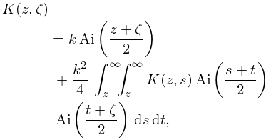
1: 32.5 Integral Equations

… ►

32.5.1 $$K(z,\zeta )=k\mathrm{Ai}\left(\frac{z+\zeta }{2}\right)+\frac{k^2}{4}{\int }_z^{\mathrm{\infty }}{\int }_z^{\mathrm{\infty }}K(z,s)\mathrm{Ai}\left(\frac{s+t}{2}\right)\mathrm{Ai}\left(\frac{t+\zeta }{2}\right)dsdt,$$

ⓘ

Symbols:

$\mathrm{Ai}\left(z\right)$: Airy function, $dx$: differential of $x$ , $\int$: integral, $z$: real, $k$: real and $K(z,\zeta )$: solution

Permalink:

http://dlmf.nist.gov/32.5.E1

Encodings:

pMML, png, TeX

See also:

Annotations for §32.5 and Ch.32

►where $k$ is a real constant, and $\mathrm{Ai}\left(z\right)$ is defined in §9.2. … ►

32.5.3 $$w(z)\sim k\mathrm{Ai}\left(z\right),$$ $z\to +\mathrm{\infty }$.

ⓘ

Symbols:

$\mathrm{Ai}\left(z\right)$: Airy function, $\sim$: asymptotic equality, $z$: real and $k$: real

Permalink:

http://dlmf.nist.gov/32.5.E3

Encodings:

pMML, png, TeX

See also:

Annotations for §32.5 and Ch.32

2: 9.19 Approximations

… ►

Martín et al. (1992) provides two simple formulas for approximating $\mathrm{Ai}\left(x\right)$ to graphical accuracy, one for , the other for .

… ►

Prince (1975) covers $\mathrm{Ai}\left(x\right)$, ${\mathrm{Ai}}^{\prime }\left(x\right)$, $\mathrm{Bi}\left(x\right)$, ${\mathrm{Bi}}^{\prime }\left(x\right)$. The Chebyshev coefficients are given to 10-11D. Fortran programs are included. See also Razaz and Schonfelder (1981).

►

Németh (1992, Chapter 8) covers $\mathrm{Ai}\left(x\right)$, ${\mathrm{Ai}}^{\prime }\left(x\right)$, $\mathrm{Bi}\left(x\right)$, ${\mathrm{Bi}}^{\prime }\left(x\right)$, and integrals ${\int }_0^x\mathrm{Ai}\left(t\right)dt$, ${\int }_0^x\mathrm{Bi}\left(t\right)dt$, ${\int }_0^x{\int }_0^v\mathrm{Ai}\left(t\right)dtdv$, ${\int }_0^x{\int }_0^v\mathrm{Bi}\left(t\right)dtdv$ (see also (9.10.20) and (9.10.21)). The Chebyshev coefficients are given to 15D. Chebyshev coefficients are also given for expansions of the second and higher (real) zeros of $\mathrm{Ai}\left(x\right)$, ${\mathrm{Ai}}^{\prime }\left(x\right)$, $\mathrm{Bi}\left(x\right)$, ${\mathrm{Bi}}^{\prime }\left(x\right)$, again to 15D.

►

Razaz and Schonfelder (1980) covers $\mathrm{Ai}\left(x\right)$, ${\mathrm{Ai}}^{\prime }\left(x\right)$, $\mathrm{Bi}\left(x\right)$, ${\mathrm{Bi}}^{\prime }\left(x\right)$. The Chebyshev coefficients are given to 30D.

… ►

Corless et al. (1992) describe a method of approximation based on subdividing $ℂ$ into a triangular mesh, with values of $\mathrm{Ai}\left(z\right)$, ${\mathrm{Ai}}^{\prime }\left(z\right)$ stored at the nodes. $\mathrm{Ai}\left(z\right)$ and ${\mathrm{Ai}}^{\prime }\left(z\right)$ are then computed from Taylor-series expansions centered at one of the nearest nodes. The Taylor coefficients are generated by recursion, starting from the stored values of $\mathrm{Ai}\left(z\right)$, ${\mathrm{Ai}}^{\prime }\left(z\right)$ at the node. Similarly for $\mathrm{Bi}\left(z\right)$, ${\mathrm{Bi}}^{\prime }\left(z\right)$.

…

3: 9.9 Zeros

… ►On the real line, $\mathrm{Ai}\left(x\right)$, ${\mathrm{Ai}}^{\prime }\left(x\right)$, $\mathrm{Bi}\left(x\right)$, ${\mathrm{Bi}}^{\prime }\left(x\right)$ each have an infinite number of zeros, all of which are negative. They are denoted by $a_k$, $a_k^{\prime }$, $b_k$, $b_k^{\prime }$, respectively, arranged in ascending order of absolute value for $k=1,2,\mathrm{\dots }.$ ► $\mathrm{Ai}\left(z\right)$ and ${\mathrm{Ai}}^{\prime }\left(z\right)$ have no other zeros. … ►For the distribution in $ℂ$ of the zeros of ${\mathrm{Ai}}^{\prime }\left(z\right)-\sigma \mathrm{Ai}\left(z\right)$, where $\sigma$ is an arbitrary complex constant, see Muraveĭ (1976) and Gil and Segura (2014). … ►Tables 9.9.1 and 9.9.2 give 10D values of the first ten real zeros of $\mathrm{Ai}$, ${\mathrm{Ai}}^{\prime }$, $\mathrm{Bi}$, ${\mathrm{Bi}}^{\prime }$, together with the associated values of the derivative or the function. …

4: 9.20 Software

… ►

§9.20(ii) $\mathrm{Ai}\left(x\right)$, ${\mathrm{Ai}}^{\prime }\left(x\right)$, $\mathrm{Bi}\left(x\right)$, ${\mathrm{Bi}}^{\prime }\left(x\right)$, $x\in ℝ$

… ►

§9.20(iii) $\mathrm{Ai}\left(z\right)$, ${\mathrm{Ai}}^{\prime }\left(z\right)$, $\mathrm{Bi}\left(z\right)$, ${\mathrm{Bi}}^{\prime }\left(z\right)$, $z\in ℂ$

… ►

§9.20(v) Integrals of $\mathrm{Ai}\left(x\right)$, $\mathrm{Bi}\left(x\right)$, $x\in ℝ$

…

5: 9.1 Special Notation

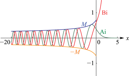
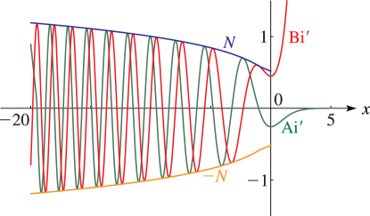
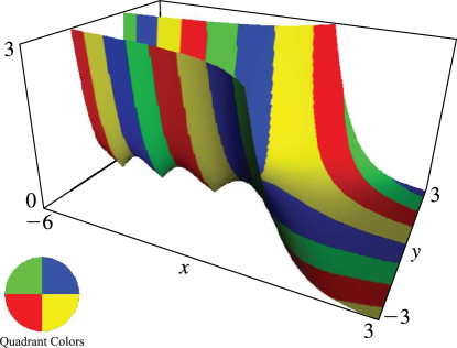
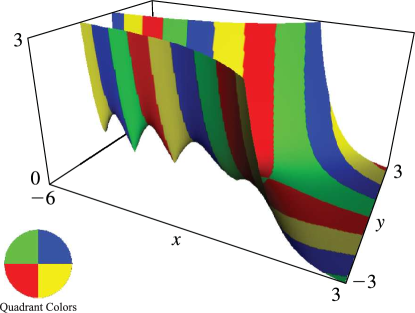
… ►The main functions treated in this chapter are the Airy functions $\mathrm{Ai}\left(z\right)$ and $\mathrm{Bi}\left(z\right)$, and the Scorer functions $\mathrm{Gi}(z)$ and $\mathrm{Hi}(z)$ (also known as inhomogeneous Airy functions). ►Other notations that have been used are as follows: $\mathrm{Ai}\left(-x\right)$ and $\mathrm{Bi}\left(-x\right)$ for $\mathrm{Ai}\left(x\right)$ and $\mathrm{Bi}\left(x\right)$ (Jeffreys (1928), later changed to $\mathrm{Ai}\left(x\right)$ and $\mathrm{Bi}\left(x\right)$); $U(x)=\sqrt{\pi }\mathrm{Bi}\left(x\right)$, $V(x)=\sqrt{\pi }\mathrm{Ai}\left(x\right)$ (Fock (1945)); $A(x)=3^{-1/3}\pi \mathrm{Ai}\left(-3^{-1/3}x\right)$ (Szegő (1967, §1.81)); $e_0(x)=\pi \mathrm{Hi}(-x)$, ${\tilde{e}}_0(x)=-\pi \mathrm{Gi}(-x)$ (Tumarkin (1959)).

6: 9.3 Graphics

… ►

►►

Figure 9.3.1: $\mathrm{Ai}\left(x\right)$, $\mathrm{Bi}\left(x\right)$, $M\left(x\right)$. … Magnify

►

►►

Figure 9.3.2: ${\mathrm{Ai}}^{\prime }\left(x\right)$, ${\mathrm{Bi}}^{\prime }\left(x\right)$, $N\left(x\right)$. … Magnify

… ►

►

►

Figure 9.3.3: $\mathrm{Ai}\left(x+\mathrm{i}y\right)$. Magnify 3D Help

… ►

►

►

Figure 9.3.5: ${\mathrm{Ai}}^{\prime }\left(x+\mathrm{i}y\right)$. Magnify 3D Help

…

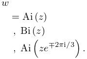
7: 9.2 Differential Equation

… ►

9.2.2 $$w=\mathrm{Ai}\left(z\right),\mathrm{Bi}\left(z\right),\mathrm{Ai}\left(z{\mathrm{e}}^{\mp 2\pi \mathrm{i}/3}\right).$$

ⓘ

Symbols:

$\mathrm{Ai}\left(z\right)$: Airy function, $\mathrm{Bi}\left(z\right)$: Airy function, $\pi$: the ratio of the circumference of a circle to its diameter, $\mathrm{e}$: base of natural logarithm, $\mathrm{i}$: imaginary unit, $z$: complex variable and $w$: ODE solution

Source:

Olver (1997b, pp. 392–393, 413–414)

Permalink:

http://dlmf.nist.gov/9.2.E2

Encodings:

pMML, png, TeX

See also:

Annotations for §9.2(i), §9.2 and Ch.9

… ►

9.2.3 $$\mathrm{Ai}\left(0\right)=\frac{1}{3^{2/3}\mathrm{\Gamma }\left(\frac{2}{3}\right)}=\mathrm{0.35502\hspace{0.33em}80538}\mathrm{\dots },$$

ⓘ

Symbols:

$\mathrm{Ai}\left(z\right)$: Airy function and $\mathrm{\Gamma }\left(z\right)$: gamma function

Source:

Olver (1997b, (1.03), p. 392)

A&S Ref:

10.4.4 (with more digits)

Permalink:

http://dlmf.nist.gov/9.2.E3

Encodings:

pMML, png, TeX

See also:

Annotations for §9.2(ii), §9.2 and Ch.9

►

9.2.4 $${\mathrm{Ai}}^{\prime }\left(0\right)=-\frac{1}{3^{1/3}\mathrm{\Gamma }\left(\frac{1}{3}\right)}=-\mathrm{0.25881\hspace{0.33em}94037}\mathrm{\dots },$$

ⓘ

Symbols:

$\mathrm{Ai}\left(z\right)$: Airy function and $\mathrm{\Gamma }\left(z\right)$: gamma function

Source:

Olver (1997b, (1.03), p. 392)

A&S Ref:

10.4.5 (with more digits)

Permalink:

http://dlmf.nist.gov/9.2.E4

Encodings:

pMML, png, TeX

See also:

Annotations for §9.2(ii), §9.2 and Ch.9

… ►

9.2.12 $$\mathrm{Ai}\left(z\right)+{\mathrm{e}}^{-2\pi \mathrm{i}/3}\mathrm{Ai}\left(z{\mathrm{e}}^{-2\pi \mathrm{i}/3}\right)+{\mathrm{e}}^{2\pi \mathrm{i}/3}\mathrm{Ai}\left(z{\mathrm{e}}^{2\pi \mathrm{i}/3}\right)=0,$$

ⓘ

Symbols:

$\mathrm{Ai}\left(z\right)$: Airy function, $\pi$: the ratio of the circumference of a circle to its diameter, $\mathrm{e}$: base of natural logarithm, $\mathrm{i}$: imaginary unit and $z$: complex variable

Source:

Olver (1997b, (8.03), p. 414)

A&S Ref:

10.4.7

Permalink:

http://dlmf.nist.gov/9.2.E12

Encodings:

pMML, png, TeX

See also:

Annotations for §9.2(v), §9.2 and Ch.9

… ►

9.2.14 $$\mathrm{Ai}\left(-z\right)={\mathrm{e}}^{\pi \mathrm{i}/3}\mathrm{Ai}\left(z{\mathrm{e}}^{\pi \mathrm{i}/3}\right)+{\mathrm{e}}^{-\pi \mathrm{i}/3}\mathrm{Ai}\left(z{\mathrm{e}}^{-\pi \mathrm{i}/3}\right),$$

ⓘ

Symbols:

$\mathrm{Ai}\left(z\right)$: Airy function, $\pi$: the ratio of the circumference of a circle to its diameter, $\mathrm{e}$: base of natural logarithm, $\mathrm{i}$: imaginary unit and $z$: complex variable

Source:

Olver (1997b, p. 414)

Permalink:

http://dlmf.nist.gov/9.2.E14

Encodings:

pMML, png, TeX

See also:

Annotations for §9.2(v), §9.2 and Ch.9

…

8: 9.11 Products

… ►For example, $w={\mathrm{Ai}}^2\left(z\right)$, $\mathrm{Ai}\left(z\right)\mathrm{Bi}\left(z\right)$, $\mathrm{Ai}\left(z\right)\mathrm{Ai}\left(z{\mathrm{e}}^{\mp 2\pi \mathrm{i}/3}\right)$, $M^2\left(z\right)$. … ►

9.11.2 $$𝒲\left\{{\mathrm{Ai}}^2\left(z\right),\mathrm{Ai}\left(z\right)\mathrm{Bi}\left(z\right),{\mathrm{Bi}}^2\left(z\right)\right\}=2{\pi }^{-3}.$$

ⓘ

Symbols:

$\mathrm{Ai}\left(z\right)$: Airy function, $\mathrm{Bi}\left(z\right)$: Airy function, $𝒲$: Wronskian, $\pi$: the ratio of the circumference of a circle to its diameter and $z$: complex variable

Proof sketch:

Use (9.2.1) and (9.2.7).

Permalink:

http://dlmf.nist.gov/9.11.E2

Encodings:

pMML, png, TeX

See also:

Annotations for §9.11(ii), §9.11 and Ch.9

… ►For an integral representation of the Dirac delta involving a product of two $\mathrm{Ai}$ functions see §1.17(ii). … ►

9.11.12 $$\int \frac{dz}{{\mathrm{Ai}}^2\left(z\right)}=\pi \frac{\mathrm{Bi}\left(z\right)}{\mathrm{Ai}\left(z\right)},$$

ⓘ

Symbols:

$\mathrm{Ai}\left(z\right)$: Airy function, $\mathrm{Bi}\left(z\right)$: Airy function, $\pi$: the ratio of the circumference of a circle to its diameter, $dx$: differential of $x$ , $\int$: integral and $z$: complex variable

Source:

Albright and Gavathas (1986, (8))

Permalink:

http://dlmf.nist.gov/9.11.E12

Encodings:

pMML, png, TeX

See also:

Annotations for §9.11(iv), §9.11(iv), §9.11 and Ch.9

►

9.11.13 $$\int \frac{dz}{\mathrm{Ai}\left(z\right)\mathrm{Bi}\left(z\right)}=\pi \ln \left(\frac{\mathrm{Bi}\left(z\right)}{\mathrm{Ai}\left(z\right)}\right),$$

ⓘ

Symbols:

$\mathrm{Ai}\left(z\right)$: Airy function, $\mathrm{Bi}\left(z\right)$: Airy function, $\pi$: the ratio of the circumference of a circle to its diameter, $dx$: differential of $x$ , $\int$: integral, $\ln z$: principal branch of logarithm function and $z$: complex variable

Source:

Albright and Gavathas (1986, (10))

Permalink:

http://dlmf.nist.gov/9.11.E13

Encodings:

pMML, png, TeX

See also:

Annotations for §9.11(iv), §9.11(iv), §9.11 and Ch.9

…

9: 9.18 Tables

… ►

Zhang and Jin (1996, p. 337) tabulates $\mathrm{Ai}\left(x\right)$, ${\mathrm{Ai}}^{\prime }\left(x\right)$, $\mathrm{Bi}\left(x\right)$, ${\mathrm{Bi}}^{\prime }\left(x\right)$ for $x=0(1)20$ to 8S and for $x=-20(1)0$ to 9D.

… ►

Woodward and Woodward (1946) tabulates the real and imaginary parts of $\mathrm{Ai}\left(z\right)$, ${\mathrm{Ai}}^{\prime }\left(z\right)$, $\mathrm{Bi}\left(z\right)$, ${\mathrm{Bi}}^{\prime }\left(z\right)$ for $\mathrm{\Re }z=-2.4(.2)2.4$, $\mathrm{\Im }z=-2.4(.2)0$. Precision is 4D.

… ►

Miller (1946) tabulates $a_k$, ${\mathrm{Ai}}^{\prime }\left(a_k\right)$, $a_k^{\prime }$, $\mathrm{Ai}\left(a_k^{\prime }\right)$, $k=1(1)50$; $b_k$, ${\mathrm{Bi}}^{\prime }\left(b_k\right)$, $b_k^{\prime }$, $\mathrm{Bi}\left(b_k^{\prime }\right)$, $k=1(1)20$. Precision is 8D. Entries for $k=1(1)20$ are reproduced in Abramowitz and Stegun (1964, Chapter 10).

►

Sherry (1959) tabulates $a_k$, ${\mathrm{Ai}}^{\prime }\left(a_k\right)$, $a_k^{\prime }$, $\mathrm{Ai}\left(a_k^{\prime }\right)$, $k=1(1)50$; 20S.

►

Zhang and Jin (1996, p. 339) tabulates $a_k$, ${\mathrm{Ai}}^{\prime }\left(a_k\right)$, $a_k^{\prime }$, $\mathrm{Ai}\left(a_k^{\prime }\right)$, $b_k$, ${\mathrm{Bi}}^{\prime }\left(b_k\right)$, $b_k^{\prime }$, $\mathrm{Bi}\left(b_k^{\prime }\right)$, $k=1(1)20$; 8D.

…

10: 9.17 Methods of Computation

… ►However, in the case of $\mathrm{Ai}\left(z\right)$ and $\mathrm{Bi}\left(z\right)$ this accuracy can be increased considerably by use of the exponentially-improved forms of expansion supplied in §9.7(v). … ►But when the integration has to be towards the origin, with starting values of $\mathrm{Ai}\left(z\right)$ and ${\mathrm{Ai}}^{\prime }\left(z\right)$ computed from their asymptotic expansions. … ►Among the integral representations of the Airy functions the Stieltjes transform (9.10.18) furnishes a way of computing $\mathrm{Ai}\left(z\right)$ in the complex plane, once values of this function can be generated on the positive real axis. … ►Gil et al. (2002c) describes two methods for the computation of $\mathrm{Ai}\left(z\right)$ and ${\mathrm{Ai}}^{\prime }\left(z\right)$ for $z\in ℂ$. …The methods for ${\mathrm{Ai}}^{\prime }\left(z\right)$ are similar. …