2人斗地主游戏大厅,网上2人斗地主游戏规则,【复制打开网址：33kk55.com】正规博彩平台,在线赌博平台,2人斗地主游戏玩法介绍,真人2人斗地主游戏规则,网上真人棋牌游戏平台,真人博彩游戏平台网址LHBxBZZZAHHQcx0Q

SearchAdvancedHelp

(0.008 seconds)

31—40 of 804 matching pages

31: 30.3 Eigenvalues

… ►With $\mu =m=0,1,2,\mathrm{\dots }$, the spheroidal wave functions ${\mathrm{𝖯𝗌}}_n^m(x,{\gamma }^2)$ are solutions of Equation (30.2.1) which are bounded on $(-1,1)$, or equivalently, which are of the form ${(1-x^2)}^{\frac{1}{2}m}g(x)$ where $g(z)$ is an entire function of $z$. These solutions exist only for eigenvalues ${\lambda }_n^m\left({\gamma }^2\right)$, $n=m,m+1,m+2,\mathrm{\dots }$, of the parameter $\lambda$. … ►The eigenvalues ${\lambda }_n^m\left({\gamma }^2\right)$ are analytic functions of the real variable ${\gamma }^2$ and satisfy … ►has the solutions $\lambda ={\lambda }_{m+2j}^m\left({\gamma }^2\right)$, $j=0,1,2,\mathrm{\dots }$. If $p$ is an odd positive integer, then Equation (30.3.5) has the solutions $\lambda ={\lambda }_{m+2j+1}^m\left({\gamma }^2\right)$, $j=0,1,2,\mathrm{\dots }$. …

32: 29.6 Fourier Series

… ►

§29.6(i) Function ${\mathrm{𝐸𝑐}}_{\nu }^{2m}(z,k^2)$

… ►In the special case $\nu =2n$, $m=0,1,\mathrm{\dots },n$, there is a unique nontrivial solution with the property $A_{2p}=0$, $p=n+1,n+2,\mathrm{\dots }$. … ►

§29.6(ii) Function ${\mathrm{𝐸𝑐}}_{\nu }^{2m+1}(z,k^2)$

… ►

§29.6(iii) Function ${\mathrm{𝐸𝑠}}_{\nu }^{2m+1}(z,k^2)$

… ►

§29.6(iv) Function ${\mathrm{𝐸𝑠}}_{\nu }^{2m+2}(z,k^2)$

…

33: 26.6 Other Lattice Path Numbers

… ► $M(n)$ is the number of lattice paths from $(0,0)$ to $(n,n)$ that stay on or above the line $y=x$ and are composed of directed line segments of the form $(2,0)$, $(0,2)$, or $(1,1)$. … ►

26.6.7 $$\sum _{n=0}^{\mathrm{\infty }}M(n)x^n=\frac{1-x-\sqrt{1-2x-3x^2}}{2x^2},$$

ⓘ

Symbols:

$n$: nonnegative integer, $M(n)$: Motzkin number and $x$: small

Referenced by:

§26.6(iii)

Permalink:

http://dlmf.nist.gov/26.6.E7

Encodings:

pMML, png, TeX

See also:

Annotations for §26.6(ii), §26.6 and Ch.26

►

26.6.8 $$\sum _{n,k=1}^{\mathrm{\infty }}N(n,k)x^n{y}^k=\frac{1-x-xy-\sqrt{{(1-x-xy)}^2-4x^{2}y}}{2x},$$

ⓘ

Symbols:

$k$: nonnegative integer, $n$: nonnegative integer, $N(n,k)$: Narayana number, $x$: small and $y$: small

Permalink:

http://dlmf.nist.gov/26.6.E8

Encodings:

pMML, png, TeX

See also:

Annotations for §26.6(ii), §26.6 and Ch.26

… ►

26.6.11 $$M(n)=M(n-1)+\sum _{k=2}^{n}M(k-2)M(n-k),$$ $n\ge 2$.

ⓘ

Symbols:

$k$: nonnegative integer, $n$: nonnegative integer and $M(n)$: Motzkin number

Referenced by:

§26.6(iii)

Permalink:

http://dlmf.nist.gov/26.6.E11

Encodings:

pMML, png, TeX

See also:

Annotations for §26.6(iii), §26.6 and Ch.26

… ►

26.6.14 $$C\left(n\right)=\sum _{k=0}^{2n}{(-1)}^k\left(\genfrac{}{}{0.0pt}{}{2n}{k}\right)M(2n-k).$$

ⓘ

Symbols:

$C\left(n\right)$: Catalan number, $\left(\genfrac{}{}{0.0pt}{}{m}{n}\right)$: binomial coefficient, $k$: nonnegative integer, $n$: nonnegative integer and $M(n)$: Motzkin number

Permalink:

http://dlmf.nist.gov/26.6.E14

Encodings:

pMML, png, TeX

See also:

Annotations for §26.6(iv), §26.6 and Ch.26

34: 29.12 Definitions

… ►The Lamé functions ${\mathrm{𝐸𝑐}}_{\nu }^m(z,k^2)$, $m=0,1,\mathrm{\dots },\nu$, and ${\mathrm{𝐸𝑠}}_{\nu }^m(z,k^2)$, $m=1,2,\mathrm{\dots },\nu$, are called the Lamé polynomials. …where $n=0,1,2,\mathrm{\dots }$, $m=0,1,2,\mathrm{\dots },n$. … ►where $\rho$, $\sigma$, $\tau$ are either $0$ or $\frac{1}{2}$. The polynomial $P(\xi )$ is of degree $n$ and has $m$ zeros (all simple) in $(0,1)$ and $n-m$ zeros (all simple) in $(1,k^{-2})$. … ►defined for $(t_1,t_2,\mathrm{\dots },t_n)$ with …

35: 34.3 Basic Properties: $\mathit{3}j$ Symbol

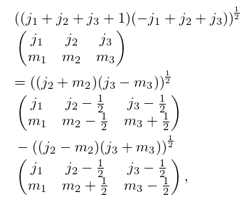
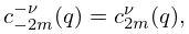
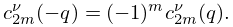
… ►When any one of $j_1,j_2,j_3$ is equal to $0,\frac{1}{2}$, or $1$, the $\mathit{3}j$ symbol has a simple algebraic form. …For these and other results, and also cases in which any one of $j_1,j_2,j_3$ is $\frac{3}{2}$ or $2$, see Edmonds (1974, pp. 125–127). … ►Even permutations of columns of a $\mathit{3}j$ symbol leave it unchanged; odd permutations of columns produce a phase factor ${(-1)}^{j_1+j_2+j_3}$, for example, … ►

34.3.13

ⓘ

Symbols:

: $\mathit{3}j$ symbol and $j,j_r$: non-negative integers or non-negative integers plus one half.

Permalink:

http://dlmf.nist.gov/34.3.E13

Encodings:

pMML, png, TeX

See also:

Annotations for §34.3(iii), §34.3 and Ch.34

… ►

34.3.15

ⓘ

Symbols:

: $\mathit{3}j$ symbol and $j,j_r$: non-negative integers or non-negative integers plus one half.

Permalink:

http://dlmf.nist.gov/34.3.E15

Encodings:

pMML, png, TeX

See also:

Annotations for §34.3(iii), §34.3 and Ch.34

…

36: 28.14 Fourier Series

… ►The coefficients satisfy ►

28.14.4 $$q{c}_{2m+2}-\left(a-{(\nu +2m)}^2\right)c_{2m}+q{c}_{2m-2}=0,$$ $a={\lambda }_{\nu }\left(q\right),c_{2m}=c_{2m}^{\nu }(q)$,

ⓘ

Symbols:

${\lambda }_{\nu +2n}\left(q\right)$: eigenvalues of Mathieu equation, $m$: integer, $q=h^2$: parameter, $\nu$: complex parameter, $a$: parameter and $c_{2m}(q)$: coefficients

Referenced by:

item (d), item (d)

Permalink:

http://dlmf.nist.gov/28.14.E4

Encodings:

pMML, png, TeX

See also:

Annotations for §28.14 and Ch.28

… ►

28.14.5 $$\sum _{m=-\mathrm{\infty }}^{\mathrm{\infty }}{\left(c_{2m}^{\nu }(q)\right)}^2=1;$$

ⓘ

Symbols:

$m$: integer, $q=h^2$: parameter, $\nu$: complex parameter and $c_{2m}(q)$: coefficients

Referenced by:

item (d)

Permalink:

http://dlmf.nist.gov/28.14.E5

Encodings:

pMML, png, TeX

See also:

Annotations for §28.14 and Ch.28

… ►

28.14.7 $$c_{-2m}^{-\nu }(q)=c_{2m}^{\nu }(q),$$

ⓘ

Symbols:

$m$: integer, $q=h^2$: parameter, $\nu$: complex parameter and $c_{2m}(q)$: coefficients

Permalink:

http://dlmf.nist.gov/28.14.E7

Encodings:

pMML, png, TeX

See also:

Annotations for §28.14 and Ch.28

►

28.14.8 $$c_{2m}^{\nu }(-q)={(-1)}^m{c}_{2m}^{\nu }(q).$$

ⓘ

Symbols:

$m$: integer, $q=h^2$: parameter, $\nu$: complex parameter and $c_{2m}(q)$: coefficients

Permalink:

http://dlmf.nist.gov/28.14.E8

Encodings:

pMML, png, TeX

See also:

Annotations for §28.14 and Ch.28

…

37: 30.16 Methods of Computation

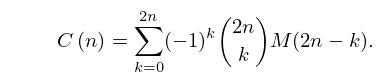
… ►and real eigenvalues ${\alpha }_{1,d}$, ${\alpha }_{2,d}$, $\mathrm{\dots }$, ${\alpha }_{d,d}$, arranged in ascending order of magnitude. … ►For $m=2$, $n=4$, ${\gamma }^2=10$, …which yields ${\lambda }_4^2\left(10\right)=\mathrm{13.97907\hspace{0.33em}345}$. … ►If ${\lambda }_n^m\left({\gamma }^2\right)$ is known, then ${\mathrm{𝖯𝗌}}_n^m(x,{\gamma }^2)$ can be found by summing (30.8.1). The coefficients $a_{n,r}^m({\gamma }^2)$ are computed as the recessive solution of (30.8.4) (§3.6), and normalized via (30.8.5). …

38: 28.4 Fourier Series

… ►For $n=0,1,2,3,\mathrm{\dots }$, … ►

$(a-4m^2)B_{2m}-q(B_{2m-2}+B_{2m+2})=0$ , $m=2,3,4,\mathrm{\dots }$, $a=b_{2n+2}\left(q\right)$, $B_{2m+2}=B_{2m+2}^{2n+2}(q).$

… ►

$B_{2n+2}^{2n+2}(0)=1,$

►

$B_{2m+2}^{2n+2}(0)=0,$ $n\ne m$.

… ►For fixed $s=1,2,3,\mathrm{\dots }$ and fixed $m=1,2,3,\mathrm{\dots }$, …

39: 19.3 Graphics

… ►

►

►

Figure 19.3.5: $\mathrm{\Pi }({\alpha }^2,k)$ as a function of $k^2$ and ${\alpha }^2$ for , $-2\le {\alpha }^2\le 2$. … Magnify 3D Help

►

►

►

Figure 19.3.6: $\mathrm{\Pi }(\varphi ,2,k)$ as a function of $k^2$ and ${\sin }^2\varphi$ for $-1\le k^2\le 3$, . Cauchy principal values are shown when ${\sin }^2\varphi >\frac{1}{2}$. … Magnify 3D Help

… ►

►

►

Figure 19.3.7: $K\left(k\right)$ as a function of complex $k^2$ for $-2\le \mathrm{\Re }\left(k^2\right)\le 2$, $-2\le \mathrm{\Im }\left(k^2\right)\le 2$. … Magnify 3D Help

►

►

►

Figure 19.3.8: $E\left(k\right)$ as a function of complex $k^2$ for $-2\le \mathrm{\Re }\left(k^2\right)\le 2$, $-2\le \mathrm{\Im }\left(k^2\right)\le 2$. … Magnify 3D Help

►

►

►

Figure 19.3.9: $\mathrm{\Re }\left(K\left(k\right)\right)$ as a function of complex $k^2$ for $-2\le \mathrm{\Re }\left(k^2\right)\le 2$, $-2\le \mathrm{\Im }\left(k^2\right)\le 2$. … Magnify 3D Help

…

40: 10.53 Power Series

… ►

10.53.1 $${𝗃}_n\left(z\right)=z^n\sum _{k=0}^{\mathrm{\infty }}\frac{{(-\frac{1}{2}{z}^2)}^k}{k!(2n+2k+1)!!},$$

ⓘ

Symbols:

$!!$: double factorial, $!$: factorial (as in $n!$), ${𝗃}_n\left(z\right)$: spherical Bessel function of the first kind, $n$: integer, $k$: nonnegative integer and $z$: complex variable

A&S Ref:

10.1.2

Referenced by:

§10.53

Permalink:

http://dlmf.nist.gov/10.53.E1

Encodings:

pMML, png, TeX

See also:

Annotations for §10.53 and Ch.10

►

10.53.2 $${𝗒}_n\left(z\right)=-\frac{1}{z^{n+1}}\sum _{k=0}^n\frac{(2n-2k-1)!!{(\frac{1}{2}{z}^2)}^k}{k!}+\frac{{(-1)}^{n+1}}{z^{n+1}}\sum _{k=n+1}^{\mathrm{\infty }}\frac{{(-\frac{1}{2}{z}^2)}^k}{k!(2k-2n-1)!!}.$$

ⓘ

Symbols:

$!!$: double factorial, $!$: factorial (as in $n!$), ${𝗒}_n\left(z\right)$: spherical Bessel function of the second kind, $n$: integer, $k$: nonnegative integer and $z$: complex variable

A&S Ref:

10.1.3

Referenced by:

§10.53

Permalink:

http://dlmf.nist.gov/10.53.E2

Encodings:

pMML, png, TeX

See also:

Annotations for §10.53 and Ch.10

►

10.53.3 $${𝗂}_n^{(1)}\left(z\right)=z^n\sum _{k=0}^{\mathrm{\infty }}\frac{{(\frac{1}{2}{z}^2)}^k}{k!(2n+2k+1)!!},$$

ⓘ

Symbols:

$!!$: double factorial, $!$: factorial (as in $n!$), ${𝗂}_n^{(1)}\left(z\right)$: modified spherical Bessel function, $n$: integer, $k$: nonnegative integer and $z$: complex variable

A&S Ref:

10.2.5

Referenced by:

§10.53

Permalink:

http://dlmf.nist.gov/10.53.E3

Encodings:

pMML, png, TeX

See also:

Annotations for §10.53 and Ch.10

►

10.53.4 $${𝗂}_n^{(2)}\left(z\right)=\frac{{(-1)}^n}{z^{n+1}}\sum _{k=0}^n\frac{(2n-2k-1)!!{(-\frac{1}{2}{z}^2)}^k}{k!}+\frac{1}{z^{n+1}}\sum _{k=n+1}^{\mathrm{\infty }}\frac{{(\frac{1}{2}{z}^2)}^k}{k!(2k-2n-1)!!}.$$

ⓘ

Symbols:

$!!$: double factorial, $!$: factorial (as in $n!$), ${𝗂}_n^{(2)}\left(z\right)$: modified spherical Bessel function, $n$: integer, $k$: nonnegative integer and $z$: complex variable

A&S Ref:

10.2.6

Referenced by:

§10.53

Permalink:

http://dlmf.nist.gov/10.53.E4

Encodings:

pMML, png, TeX

See also:

Annotations for §10.53 and Ch.10

►For ${𝗁}_n^{(1)}\left(z\right)$ and ${𝗁}_n^{(2)}\left(z\right)$ combine (10.47.10), (10.53.1), and (10.53.2). …